In this tutorial we begin with a new genome assembly just produced in the Unicycler tutorial. This is an assembly of E. coli C, which we will be comparing to assemblies of all other complete genes of this species.
E. coli is one of the most studied organisms. There are thousands of complete genomes (in fact, the total number of E. coli assemblies in Genbank is over 10,500). Here we will shows how to uploaded all (!) complete E. coli genomes at once.
Comment: Slow steps ahead
The first part of this tutorial can take a significant amount of time to find the most related genomes. If you want, you can upload this (outdated) copy of the NCBI E. Coli Genomes table to your history:
Our initial objective is to compare our assembly against all complete E. coli genomes to identify the most related ones and to find any interesting genome alterations. In order to do this we need to align our assembly against all other genomes. And in order to do that we need to first obtain all these other genomes.
NCBI is the resource that would store all complete E. coli genomes. This list contains over 500 genomes and so uploading them by hand will likely result in carpal tunnel syndrome, which we want to prevent. Galaxy has several features that are specifically designed for uploading and managing large sets of similar types of data. The following two Hands-on sections show how they can be used to import all completed E. coli genomes into Galaxy.
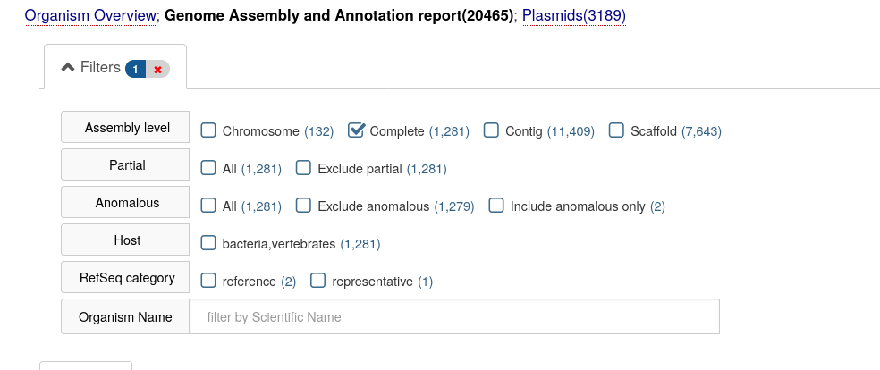
Hands On: Preparing a list of all complete E. coli genomes
For this tutorial we made this dataset available from Zenodo, but it is of course also possible to obtain the data directly from NCBI.
Note that the format of the files on NCBI may change, which means some of the parameter settings of tools in this tutorial will need
to be altered (e.g. column numbers) when using data directly from NCBI.
Below we describe how you could obtain this data from NCBI.
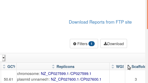
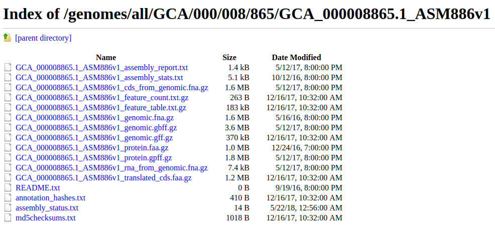
Now that the list is formatted as a table in a spreadsheet, it is time to upload it into Galaxy. There is a problem though: the URLs (web addresses) in the list do not actually point to sequence files that we would need to perform alignments. Instead they point to directories. For example, this URL: GCA_000008865.1_ASM886v1 points to a directory (rather than a file) containing many files, most of which we do not need.
Figure 1: A list of files for an E. coli assembly. For further analyses we only need the dataset ending with _genomic.fna.gz.
So to download sequence files we need to edit URLs by adding filenames to them. For example, in the case of the URL shown above we need to add /GCA_000008865.1_ASM886v1 and _genomic.fna.gz to the end to get this:
This can be done as a two step process where we first copy the end part of the existing URL (/GCA_000008865.1_ASM886v1) and then add a fixed string _genomic.fna.gz to the end of it. Doing this by hand is crazy and trying to do it in a spreadsheet is complicated. Fortunately, Galaxy’s new rule-based uploader can help, as shown in the next Hands-on section:
Hands On: Data upload
Again Uploadtool data
Switch to the Rule-based tab on the right
There is a detailed tutorial on using the Rule based Uploader if you want to learn about the more advanced features available.
“Upload data as”: Collection(s)
“Load tabular data from”: History Dataset
“Select dataset to load”: output of the cut tool
If the dataset doesn’t appear in the select list, refresh your page.
From Column, select Using a Regular Expression
“From Column”: B
Select Create columns matching expression groups
“Regular Expression”: .*(\/GCA.*$)
“Number of Groups”: 1
Click Apply
From Column, select Concatenate Columns
“From Column”: B
“From Column”: C
Click Apply
From Column, select Fixed Value
“Value”: _genomic.fna.gz
Click Apply
From Column, select Concatenate Columns
“From Column”: D
“From Column”: E
Click Apply
From Rules menu, select Add / Modify Column Definitions
Add Definition, List Identifier(s), Select Column A
Add Definition, URL, Column F
Click Apply
Set the Type in the bottom left to fasta.gz
Give the upload a name like Complete genomes
Upload
Now we have all complete E. coli genomes in Galaxy’s history. It is time to do a few things to our assembly.
Preparing assembly
Before starting any analyses we need to upload the assembly produced in Unicycler tutorial from Zenodo:
Hands On: Uploading E. coli assembly into Galaxy
Upload :
Click Paste/Fetch data button (Bottom of the interface box)
Pastehttps://zenodo.org/record/1306128/files/Ecoli_C_assembly.fna into the box.
“Type”: fasta
Click Start
Galaxy instances contain hundreds of tools. As a result, it can be hard to find tools mentioned in tutorials such as this one. To help with this challenge, Galaxy has a search box at the top of the left panel. Use this box to find the tools mentioned here.
The assembly we just uploaded has two issues that need to be addressed before proceeding with our analysis:
It contains two sequences: the one of E. coli C genome (the one we really need) and another representing phage phiX174 (a by product of Illumina sequencing where it is used as a spike-in DNA).
Sequences have unwieldy names like >1 length=4576293 depth=1.00x circular=true. We need to rename it to something more meaningful.
Let’s fix these two problems.
Because phiX173 is around 5,000bp, we can remove those sequences by setting a minimum length of 10,000:
Hands On: Fixing assembly
Filter sequences by length ( Galaxy version 1.2) with the following parameters:
“Fasta file”: the dataset you’ve just uploaded. (https://zenodo.org/record/1306128/files/Ecoli_C_assembly.fna).
“Minimal length”: 10000
Replace Text ( Galaxy version 1.1.2) in entire line:
“File to process”: the output of the Filter sequences by length tool
“1: Replacement”
“Find Pattern”: ^>1.*
“Replace with”: >Ecoli_C
Click on the galaxy-pencilpencil icon for the dataset to edit its attributes
In the central panel, change the Name field to E. coli C
The expression ^>1.* contains several pieces that you need to understand. Let’s write it top-to-bottom and explain:
^ - says start looking at the beginning of each line
> - is the first character we want to match. Remember that name of the sequence in FASTA files starts with >
1 - is the number present is our old name (>1 length=4576293 depth=1.00x circular=true to >Ecoli_C)
. - dot has a special meaning. It signifies any character
* - is a quantifier. From Wikipedia: “The asterisk indicates zero or more occurrences of the preceding element. For example, ab*c matches ac, abc, abbc, abbbc, and so on.”
So in short we are replacing >1 length=4576293 depth=1.00x circular=true with >Ecoli_C. The Regular expression^>1.* is used here to represent >1 length=4576293 depth=1.00x circular=true.
Detailed description of regular expressions is outside of the scope of this tutorial, but there are other great resources. Start with Software Carpentry Regular Expressions tutorial.
Question
What is the meaning of ^ character is SED expression?
It tells SED to start matching from the beginning of the string.
Generating alignments
Now everything is loaded and ready to go. We will now align our assembly against each of the E. coli genomes we have uploaded into the collection. To do this we will use LASTZ—an aligner designed for long sequences.
Hands On: Running LASTZ
LASTZ ( Galaxy version 1.3.2) with the following parameters:
“Select TARGET sequence(s) to align against”: from your history
param-collection“Select a reference dataset”: the “Complete genomes” collection we uploaded earlier
param-file“Select QUERY sequence(s)”: our E. coli assembly which was prepared in the previous step.
Chaining
“Perform chaining of HSPs with no penalties”: Yes
Output
“Specify the output format”: blastn
Note that because we started LASTZ on a collection of E. coli genomes, it will output alignment information as a collection as well. A collection is simply a way to represent large sets of similar data in a compact way within Galaxy’s interface.
Warning: It will take a while!
Please understand that alignment is not an instantaneous process: allow several hours for these jobs to clear.
Finding closely related assemblies
Understanding LASTZ output
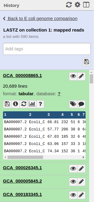
LASTZ produced data in so-called blastn format (because we explicitly told LASTZ to output in this format, see previous step), which looks like this:
The alignment information produced by LASTZ is a collection. In this collection each element contains alignment data between each of the E. coli genomes and our assembly:
Figure 3: LASTZ produced a collection where each element corresponds to an alignment between an E. coli genome and our assembly. Here one of the elements is expanded (to expand an element simply click on it).
.
Collapsing collection
Collections are a wonderful way to organize large sets of data and parallelize data processing like we did here with LASTZ. However, at this point we need to combine all data into one dataset. Follow the steps below to accomplish this:
Hands On: Combining collection into a single dataset
Collapse Collection ( Galaxy version 4.2) with the following parameters:
“Collection of files to collapse”: the output of LASTZ (collecion input)
This will produce one gigantic table (over 12 million lines) containing combined LASTZ output for all genomes.
Getting taste of the alignment data
To make further analyses we need to get an idea about alignment data generated with LASTZ. To do this let’s select a random subsample of the large dataset we’ve generated above. This is necessary because processing the entire dataset will take time and will not give us a better insight anyway. So first we will select 10,000 lines from the alignment data:
Hands On: Selecting random subset of data
Select random lines from a file with the following parameters:
“Randomly select”: 10000
“from”: the output from Collapse Collection
Now we can visualize this dataset to discover generalities:
Hands On: Graphing alignment data
Expand random subset of alignment data generated on the previous step by clicking on it.
You will see “chart” button galaxy-barchart. Click on it.
In the central panel you will see a list of visualizations. Select Scatter plot (NVD3)
Click Select datagalaxy-chart-select-data
Set Values for x-axis to Column: 3 (alignment identity)
Set Values for y-axis to Column: 4 (alignment length)
You can also click on configuration button galaxy-gear and specify axis labels etc.
The relationship between the alignment identity and alignment length looks like this (remember that this is only a subsample of the data):
Figure 4: Alignment identity (%) versus length (bp). This graph is truncated at the top
You can see that most alignments are short and have relatively low identity. Thus we can filter the original dataset by identity and length. Judging from this graph we can select alignment longer than 10,000 bp with identity above 90%.
Hands On: Filtering data
Filter data on any column using simple expressions:
“Filter”: the full dataset, from the output of the Collapse Collectiontool.
“With following condition”: c3 >= 90 and c4 >= 10000 (here c stands for column).
Remember, our objective is to find the genomes that are most similar to ours. Given the alignment data in the table we just created we can define similarity as follows:
Genomes that have the smallest number of alignment blocks but the highest overall alignment length are most similar to our assembly. This essentially means that they have longest uninterrupted region of high similarity to our assembly.
However, to extract this information from our data we need to aggregate it. In other words, for each E. coli genome we need to calculate the total number of alignment blocks, their combined length, and average identity. The following section explains how to do this:
Hands On: Aggregating the data
Datamash (operations on tabular data) ( Galaxy version 1.1.0) with the following parameters:
“Input tabular dataset”: output of the previous Filter step.
“Group by fields”: 2. (column 1 contains name of the E. coli genome we mapped against)
“Sort input”: Yes
“Operation to perform on each group”:
“Type”: Count
“On column”: Column: 2
param-repeat“Insert operation to perform on each group”
“Operation to perform on each group”:
“Type”: Mean
“On column”: Column: 3.
param-repeat“Insert operation to perform on each group”
“Operation to perform on each group”:
“Type”: Sum
“On column”: Column: 4
Finding closest relatives
The dataset generated above lists each E. coli genome accession only once and will have aggregate information for the number of alignment blocks, mean identity, and total length. Let’s graph these data:
Hands On: Graphing aggregated data
Expand the aggregated data generated on the previous step by clicking on it.
You will see “chart” button galaxy-barchart. Click on it.
In the central panel you will see a list of visualizations. Select Scatter plot (NVD3)
Click Select datagalaxy-chart-select-data
Set Data point labels to Column: 1 (Accession number of each E. coli genome)
Set Values for x-axis to Column: 2 (# of alignment blocks)
Set Values for y-axis to Column: 4 (Total alignment length)
You can also click on configuration button galaxy-gear and specify axis labels etc.
The relationship between the number of alignment blocks and total alignment length looks like this:
Figure 5: Number of alignment blocks versus total alignment length (bp).
A group of three dots in the upper left corner of this scatter plot represents genomes that are most similar to our assembly: they have a SMALL number of alignment blocks but HIGH total alignment length. Mousing over these three dots (if you set Data point labels correctly in the previous step) will reveal their accession numbers: LT906474.1, CP024090.1, and CP020543.1.
Warning: Things change
It is possible that when you repeat these steps the set of sequences in NCBI will have changed and you will obtain different accession numbers. Keep this in mind.
Let’s find table entries corresponding to these:
Hands On: Extracting into about best hits
Select lines that match an expression with the following parameters:
“Select lines from”: to the output from Datamash
“the pattern”: LT906474|CP024090|CP020543. (Here | means or).
This will generate a short table like this:
CP020543.1
11
99.926363636364
4486976
CP024090.1
12
99.911666666667
4540487
LT906474.1
8
99.94
4575200
From this it appears that LT906474.1 is closest to our assembly because it has eight alignment blocks, the longest total alignment length (4,575,223) and highest mean identity (99.94%).
Comparing genome architectures
Now that we know the three genomes most closely related to ours, let’s take a closer look at them. First we will re-download sequence and annotation data.
Getting sequences and annotations
Hands On: Uploading sequences and annotations
Using the three accession listed above we will fetch necessary data from NCBI. We will use the spreadsheet we uploaded at the start to accomplish this.
Upload the E. coli C genome if you have not done so already:
Click Paste/Fetch data button (Bottom of the interface box)
Pastehttps://zenodo.org/record/1306128/files/Ecoli_C_assembly.fna into the box.
“Type”: fasta
Click Start
Select lines that match an expression with the following parameters:
“Select lines from”: the genomes.tsv you uploaded earlier
You can click the tool next to the header Rulestool, and paste the contents there, before clicking Apply, checking “Add nametag for name” and then Upload.
From Column, select Using a Regular Expression
“From Column”: B
Select Create columns matching expression groups
“Regular Expression”: .*(\/GCA.*$)
“Number of Groups”: 1
Click Apply
From Column, select Concatenate Columns
“From Column”: B
“From Column”: C
Click Apply
From Rules, select Remove Columns(s)
“From Column”: B, C
Click Apply
From Column, select Fixed Value
“Value”: _feature_table.txt.gz
Click Apply
From Column, select Fixed Value
“Value”: _genomic.fna.gz
Click Apply
From Column, select Concatenate Columns
“From Column”: B
“From Column”: C
Click Apply
From Column, select Concatenate Columns
“From Column”: B
“From Column”: D
Click Apply
From Rules, select Remove Columns(s)
“From Column”: B, C, D
Click Apply
From Column, select Fixed Value
“Value”: Genes
Click Apply
From Column, select Fixed Value
“Value”: DNA
Click Apply
From Column, select Using a Regular Expression
“From Column”: B
Select Create columns matching expression groups
“Regular Expression”: .*\/(.*)
“Number of Groups”: 1
Click Apply
From Rules menu, select Swap Column(s)
“Swap Column”: A
“With Column”: F
Click Apply
From Rules, select Remove Columns(s)
“From Column”: F
Click Apply
From Rules menu, select Split Column(s)
“Odd Row Column(s)”: B, D
“Even Row Column(s)”: C, E
Click Apply
From Rules menu, select Add / Modify Column Definitions
Add Definition, List Identifier(s), Select Column A
Add Definition, URL, Column B
Add Definition, Collection Name, Column C
Click Apply
Check Add nametag for name
Upload
At the end of this you should have two collections: one containing genomic sequences and another containing annotations.
Visualizing rearrangements
Now we will perform alignments between our assembly and the three most closely related genomes to get a detailed look at any possible genome architecture changes. We will again use LASTZ:
Hands On: Aligning again
LASTZ ( Galaxy version 1.3.2) with the following parameters:
“Select TARGET sequence(s) to align against”: from your history
param-collection“Select a reference dataset”: DNA, the E. coli genomes we uploaded earlier
param-file“Select QUERY sequence(s)”: E. coli C fasta file
“Select which fields to include”: select the following
score alignment score
name1 name of the target sequence
strand1 strand for the target sequence
zstart1 0-based start of alignment in target
end1 end of alignment in target
length1 length of alignment in target
name2 name of query sequence
strand2 strand for the query sequence
zstart2 0-based start of alignment in query
end2 end of alignment in query
identity alignment identity
number alignment number
“Create a dotplot representation of alignments?”: Yes
Rename the LASTZ on collection... mapped reads something more memorable like LASTZ Alignments
Click on the collection
Click on the name of the collection at the top
Change the name to LASTZ Alignments
Press Enter
Because we chose to produce Dot Plots as well, LASTZ will generate two collections: one containing alignment data and the other containing DotPlots in PNG format:
Figure 6: Dot Plot representations of alignments between three E. coli genomes and our assembly. Target (X-axis) is indicated above each dot plot. Query (Y-axis) is our assembly. Red circle indicates a region deleted in our assembly.
A quick conclusion that can be drawn here is that there is a large inversion in CP020543 and deletion in our assembly.
If you are not sure how to interpret Dot Plots here is a great explanation by Michael Schatz:
Figure 7: A quick reference to interpreting Dot Plots. Our case is identical to Insertion into Reference shown in the upper left.
For a moment let’s leave LASTZ result and create a browser that would allows us to display our results.
Producing a Genome Browser for this experiment
The dot plots we’ve produced above are great, but they are static. It would be wonderful to load these data into a genome browser where one can zoom in and out as well as add tracks such as those containing genes. To create a browser we need a genome and a set of tracks. Tracks are features such as genes or SNPs with start and end positions corresponding to a coordinate system provided by the genome. Thus the first thing to do is to create a genome that would represent our experiment. We can create such a genome by simply combining the three genomes of closely related strains with our assembly in a single dataset—a hybrid genome.
Collecting the genomes
The first step will be collapsing the collection containing the three genomes into a single file:
Hands On: Creating a single FASTA dataset with all genomes
Collapse Collection ( Galaxy version 4.0)
param-collection“Collection of files to collapse” the three genomes (collection) named DNA
Convert the datatype of this output to uncompress it
Click on the galaxy-pencil pencil icon for the dataset to edit its attributes.
In the central panel, click galaxy-chart-select-data Datatypes tab on the top.
In the galaxy-gear Convert to Datatype section, select Convert compressed to uncompressed from “Target datatype” dropdown.
Click the Create Dataset button to start the conversion.
Concatenate datasets ( Galaxy version 0.1.0) tail-to-head (cat):
“Datasets to concatenate”: Collapse collection ... uncompressed, the output from the uncompression step.
Click Insert Dataset button
“Select”: the E. coli C file from the start of the history
Rename the output to DNA (E. coli C + Relatives)
Click on the galaxy-pencilpencil icon for the dataset to edit its attributes
In the central panel, change the Name field to DNA (E. coli C + Relatives)
Click the Save button
The resulting dataset contains four sequences: three genomes plus our assembly.
Preparing the alignments
Above we computed alignments using LASTZ. Because we ran LASTZ on a collection containing genomic sequences, LASTZ produced a collection as well (actually two collections: one containing alignments an the other with dot plots). To display alignments in the browser we need to do several things:
Create a single BED track containing alignments against all four genomes.
To begin, let’s look at the LASTZ output:
1
2
3
4
5
6
7
8
9
10
11
12
13
10141727
CP020543.1
+
48
106157
106109
Ecoli_C
+
0
106109
106107/106109
100.0%
1
5465
CP020543.1
+
121267
121367
100
Ecoli_C
+
109317
109418
76/100
76.0%
2
4870
CP020543.1
+
159368
159512
144
Ecoli_C
+
128706
128828
95/115
82.6%
3
One immediate problem is % character in column 12 (alignment identity). We need to remove it as we will use this for the score column of the BED file, and that must be a normal number and not a percentage.
Column 13 of the fields chosen by us for LASTZ run is number. This is an incrementing number given by LASTZ to every alignment block so it can be uniquely identified. The problem is that by running LASTZ on a collection of three genomes it generated a number for each output independently starting with 1 each time. So these alignments identified are unique within each individual run but are redundant for multiple runs. We can fix that by pre-pending each alignment identified (column 12) with the name of the target sequence (column 2). This would create alignments that are truly unique. For example, in the case of the LASTZ output shown above alignment identifier 1 will become CP020543.11, 2 will become CP020543.12 and so on.
Comment: BED format
Our goal is to convert this into a format that will be acceptable to the genome browser. One of such formats is BED. In one of its simplest forms (there is one even simpler - 3 column BED) it has six columns:
Chromosome ID
Start
End
Name of the feature
Score (must be between 0 and 1000)
Strand (+, -, or . for no strand data).
Hands On: Convert LASTZ output to BED
Replace Text ( Galaxy version 1.1.0) in a specific column:
param-collection“File to process”: output of LASTZ (LASTZ Alignments)
“in column”: Column 12
“Find pattern”: %
“Replace with”: leave empty
Merge Columns together ( Galaxy version 1.0.1) with the following parameters:
param-collection“Select data”: the output of the previous step, Replace Text on collection ...
“Merge column”: Column: 2 (this is the Target sequence name)
“with column”: Column: 13 (this is the alignment block created by LASTZ)
The tool added a new column (Column 14) containing a merge between the target name and alignment id. Now we can differentiate between alignment blocks that exist between, for example, CP020543.1 and LT906474.1 because they will have accessions embedded within alignment block IDs. For example, the first alignment between CP020543.1 and our assembly Ecoli_C will have alignment block id CP020543.11, while the 225th alignment between LT906474.1 and Ecoli_C will have ID LT906474.1225. Because of this we can collapse the entire collection of alignments into a single dataset:
Collapse Collection ( Galaxy version 4.0) with the following parameters:
param-collection“Collection of files to collapse”: the output of the previous step, Merge Columns on collection...
This will produce a single dataset combining all alignment info. We can tell which alignments are between which genomes because we have set identifiers such as CP020543.13.
We will reuse this file later so let’s rename it Unprocessed Alignments
Click on the galaxy-pencilpencil icon for the dataset to edit its attributes
In the central panel, change the Name field to Unprocessed Alignments
Click the Save button
Cut columns from a table:
“Cut columns”: c2,c4,c5,c14,c12,c8
param-file“From”: the output of the previous step (Unprocessed alignments)
Let’s look again at the data we generated in the last step:
1
2
4
4
5
6
7
8
9
10
11
12
13
14
10141727
CP020543.1
+
48
106157
106109
Ecoli_C
+
0
106109
106107/106109
100.0
1
CP020543.11
5465
CP020543.1
+
121267
121367
100
Ecoli_C
+
109317
109418
76/100
76.0
2
CP020543.12
4870
CP020543.1
+
159368
159512
144
Ecoli_C
+
128706
128828
95/115
82.6
3
CP020543.13
Alignments are regions of high similarity between two sequences. Therefore each alignment block has two sets of coordinates associated with it: start/end in the first sequences (target) and start/end in the second sequence (query). But BED only has one set of coordinates. Thus we can create two BEDs: one using coordinates from the target and the other one from query. The first file will depict alignment data from the standpoint of target sequences CP020543.1, CP024090.1, LT906474.1 and the second from the standpoint of query - our own assembly we calledEcoli_C.
In the first BED, column 1 will contain names of targets (CP020543.1, CP024090.1, and LT906474.1).
In the second BED, column 1 will contain name of our assembly: Ecoli_C.
To create the first BED we will cut six columns from the dataset produced at the last step. Specifically, to produce the target BED we will cut columns 2, 4, 5, 14, 12, and 8. To produce the query BED columns 7, 9, 10, 14, 12, 8 will be cut.
Warning: There are multiple CUT tools!
The Hands-On box below uses Cut tool. Beware that some Galaxy instances contain multiple Cut tools. The one that is used below is called Cut columns from a table while the other one, which we will NOT use is called Cut columns from a table (cut). It is a small difference, but the tools are different.
This will produce a dataset looking like this:
1
2
3
4
5
6
CP020543.1
48
106157
CP020543.11
100.0
+
CP020543.1
121267
121367
CP020543.12
76.0
+
CP020543.1
159368
159512
CP020543.13
82.6
+
Depending on the steps and other choices, the genomes may be in a different order here. This is unimportant, as all of the same alignments are contained in the file, just the ordering is different. As long as these columns look correct (start/end in column 2/3 are reasonable, a number between 0-100 in column 5, and a + or - in column 6) then it is OK.
Rename this “Target Alignments”
Click on the galaxy-pencilpencil icon for the dataset to edit its attributes
In the central panel, change the Name field to Target Alignments
Click the Save button
Cut columns from a table with the following parameters
“Cut columns”: c7,c9,c10,c14,c12,c8 (look at the data shown above and the definition of BED to see why we make these choices.)
“From”: Unprocessed alignments, the output of collection collapse
Rename this “Query Alignments”
Click on the galaxy-pencilpencil icon for the dataset to edit its attributes
In the central panel, change the Name field to Query Alignments
Click the Save button
Concatenate multiple datasets or collections
“Concatenate Dataset”: Query Alignments
Click “Insert Dataset” button
“1: Dataset”: Target Alignments
Change the datatype of the output to BED and rename the output “Target & Query Alignments”
Click on the galaxy-pencilpencil icon for the dataset to edit its attributes
In the central panel, click galaxy-chart-select-dataDatatypes tab on the top
In the galaxy-chart-select-dataAssign Datatype, select bed from “New Type” dropdown
Tip: you can start typing the datatype into the field to filter the dropdown menu
Click the Save button
Click on the galaxy-pencilpencil icon for the dataset to edit its attributes
In the central panel, change the Name field to Target & Query Alignments
Click the Save button
This will produce a dataset looking like this:
1
2
3
4
5
6
Ecoli_C
0
106109
CP020543.11
100.0
+
Ecoli_C
109317
109418
CP020543.12
76.0
+
Ecoli_C
128706
128828
CP020543.13
82.6
+
Extracting Genes
Earlier we downloaded gene annotations for the three genomes most closely related to our assembly. The data was downloaded as a collection containing annotations for CP020543.1, CP024090.1, and LT906474.1. The annotation data contains multiple columns described by NCBI as follows (you can look at the actual data by finding the annotation collection from above (called Genes)):
Tab-delimited text file reporting locations and attributes for a subset of
annotated features. Included feature types are: gene, CDS, RNA (all types),
operon, C/V/N/S_region, and V/D/J_segment.
The file is tab delimited (including a #header) with the following columns:
Column
Definition
1
feature: INSDC feature type
2
class: Gene features are subdivided into classes according to the gene biotype computed based on the set of child features for that gene. See the description of the gene_biotype attribute in the GFF3 documentation for more details: ftp://ftp.ncbi.nlm.nih.gov/genomes/README_GFF3.txt ncRNA features are subdivided according to the ncRNA_class. CDS features are subdivided into with_protein and without_protein, depending on whether the CDS feature has a protein accession assigned or not. CDS features marked as without_protein include CDS features for C regions and V/D/J segments of immunoglobulin and similar genes that undergo genomic rearrangement, and pseudogenes.
3
assembly: assembly accession.version
4
assembly_unit: name of the assembly unit, such as “Primary Assembly”, “ALT_REF_LOCI_1”, or “non-nuclear”
5
seq_type: sequence type, computed from the “Sequence-Role” and “Assigned-Molecule-Location/Type” in the *_assembly_report.txt file. The value is computed as: if an assembled-molecule, then reports the location/type value. e.g. chromosome, mitochondrion, or plasmid if an unlocalized-scaffold, then report “unlocalized scaffold on ". e.g. unlocalized scaffold on chromosome else the role, e.g. alternate scaffold, fix patch, or novel patch
6
chromosome
7
genomic_accession
8
start: feature start coordinate (base-1). start is always less than end
9
end: feature end coordinate (base-1)
10
strand
11
product_accession: accession.version of the product referenced by this feature, if exists
12
non-redundant_refseq: for bacteria and archaea assemblies, the non-redundant WP_ protein accession corresponding to the CDS feature. May be the same as column 11, for RefSeq genomes annotated directly with WP_ RefSeq proteins, or may be different, for genomes annotated with genome-specific protein accessions (e.g. NP_ or YP_ RefSeq proteins) that reference a WP_ RefSeq accession.
13
related_accession: for eukaryotic RefSeq annotations, the RefSeq protein accession corresponding to the transcript feature, or the RefSeq transcript accession corresponding to the protein feature.
14
name: For genes, this is the gene description or full name. For RNA, CDS, and some other features, this is the product name.
15
symbol: gene symbol
16
GeneID: NCBI GeneID, for those RefSeq genomes included in NCBI’s Gene resource
17
locus_tag
18
feature_interval_length: sum of the lengths of all intervals for the feature (i.e. the length without introns for a joined feature)
19
product_length: length of the product corresponding to the accession.version in column 11. Protein product lengths are in amino acid units, and do not include the stop codon which is included in column 18. Additionally, product_length may differ from feature_interval_length if the product contains sequence differences vs. the genome, as found for some RefSeq transcript and protein products based on mRNA sequences and also for INSDC proteins that are submitted to correct genome discrepancies.
20
attributes: semi-colon delimited list of a controlled set of qualifiers. The list currently includes: partial, pseudo, pseudogene, ribosomal_slippage, trans_splicing, anticodon=NNN (for tRNAs), old_locus_tag=XXX
Our objective is to convert these data into BED. In this analysis we want to initially concentrate on protein coding regions. To do this let’s select all lines from the annotation datasets that contain the term CDS, then
we will produce a collection with three datasets just like the original Genes collection but containing only CDS data. Next we need to cut out only those columns that need to be included in the BED format. There is one problem with this. We are trying to convert these data into 6 column BED. In this format the fifth column (score) must have a value between 0 and 1000. To satisfy this requirement we will create a dummy column that will always have a value of 0.
Finally we can cut necessary columns from these datasets. These columns are 8 (start), 9 (end), 15 (gene symbol), 21 (dummy column we just created), and c10 (strand), and then we can add the genome name.
Hands On: Extract CDSs from annotation datasets
Select lines that match an expression with the following parameters:
param-collection“Select lines from”: the collection containing annotations, Genes
“the pattern”: ^CDS
This is because we want to retain all lines that begin (^) with CDS.
Add column to an existing dataset ( Galaxy version 1.0.0) with the following parameters:
“Add this value”: 0
param-collection“to Dataset”: the collection produced by the previous step (Select on collection...)
This will be used for the “score” field of the BED file since we do not have a proper “score”
Cut columns from a table with the following parameters:
We will produce two BED files, one using the product name (e.g. “chromosomal replication initiator protein DnaA”) and one using the symbol (e.g. “thrA”). The product name is much more interesting to see in visualisations, but the symbol is more often used in other analyses and we will use that file later. We will start with the product name:
“Cut columns”: c8,c9,c14,c21,c10
param-collection“From” the collection produced at the previous step (Add column on collection...)
This will produce a collection with each element containing data like this:
1
2
3
4
5
49
1452
chromosomal replication initiator protein DnaA
0
+
1457
2557
DNA polymerase III subunit beta
0
+
2557
3630
DNA replication and repair protein RecF
0
+
As we mentioned above these datasets lack genome IDs such as CP020543.1. However, the individual elements in the collection we’ve created already have genome IDs. We will leverage this when collapsing this collection into a single dataset:
Collapse Collection ( Galaxy version 4.2) with the following parameters:
“Collection of files to collapse”: the output of the previous step (Cut on collection...)
“Prepend File name”: Yes
“Where to add dataset name”: Same line and each line in dataset
Replace Text ( Galaxy version 1.1.3) in a specific column
Many bed parsers do not like whitespace in the Name column, so we will replace that
param-collection“File to process”: output of the previous Collapse Collectiontool step
“in column”: Column 4
“Find pattern”: [^A-Za-z0-9_-] (any character that isn’t a number or letter or underscore or minus)
“Replace with”: _
Change the datatype of the collection to bed and rename it to Genes (E. coli Relatives)
Click on the galaxy-pencilpencil icon for the dataset to edit its attributes
In the central panel, click galaxy-chart-select-dataDatatypes tab on the top
In the galaxy-chart-select-dataAssign Datatype, select bed from “New Type” dropdown
Tip: you can start typing the datatype into the field to filter the dropdown menu
Click the Save button
Click on the galaxy-pencilpencil icon for the dataset to edit its attributes
In the central panel, change the Name field to Genes (E. coli Relatives)
Click the Save button
Question
How does your output look?
The resulting dataset should look like this:
1
2
3
4
5
6
CP020543.1
49
1452
chromosomal_replication_initiator_protein_DnaA
0
+
CP020543.1
1457
2557
DNA_polymerase_III_subunit_beta
0
+
CP020543.1
2557
3630
DNA_replication_and_repair_protein_RecF
0
+
You can see that the genome ID is now appended at the beginning and this dataset looks like a legitimate BED that can be visualized.
For the BED file with the symbol:
Cut columns from a table with the following parameters:
We will produce two BED files, one using the product name (e.g. “chromosomal replication initiator protein DnaA”) and one using the symbol (e.g. “thrA”). The product name is much more interesting to see in visualisations, but the symbol is more often used in other analyses and we will use that file later. We will start with the product name:
“Cut columns”: c8,c9,c15,c21,c10
param-collection“From” the collection produced at the previous step (Add column on collection...)
This will produce a collection with each element containing data like this:
1
2
3
4
5
49
1452
dnaA
0
+
1457
2557
0
+
2557
3630
0
+
Collapse Collection ( Galaxy version 4.0) with the following parameters:
“Collection of files to collapse”: the output of the previous step (Cut on collection...)
“Append File name”: Yes
“Where to add dataset name”: Same line and each line in dataset
Change the datatype of the collection to bed and rename it to Genes (E. coli Relatives) with Symbol Name
Click on the galaxy-pencilpencil icon for the dataset to edit its attributes
In the central panel, click galaxy-chart-select-dataDatatypes tab on the top
In the galaxy-chart-select-dataAssign Datatype, select bed from “New Type” dropdown
Tip: you can start typing the datatype into the field to filter the dropdown menu
Click the Save button
Click on the galaxy-pencilpencil icon for the dataset to edit its attributes
In the central panel, change the Name field to Genes (E. coli Relatives) with Symbol Name
Click the Save button
Extracting Gap Regions
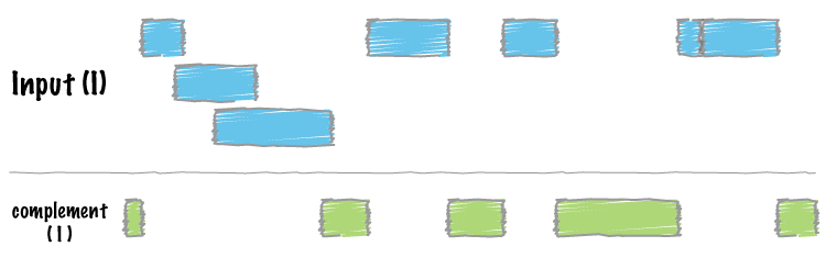
It can be useful to have the complement of the aligned regions, to know which regions are unique.
Figure 8: Any set of genomic intervals can complemented or converted into a set of intervals that do not overlap the original set (image from BEDTools documentation).
Hands On: Creating a genome file
Compute sequence length ( Galaxy version 1.0.1):
param-file“Compute length for these sequences”: DNA (E. coli + Relatives), the FASTA dataset we generated from Collapse Collectiontool
“Strip fasta description from header”: Yes
Sort ( Galaxy version 1.1.1) data in ascending or descending order:
param-file“Sort Dataset”: the output of the previous step (Compute sequence length on ...)
“on column”: Column: 1
“with flavor”: Alphabetical sort
“everything in”: Ascending order
Question
How does the output look?
This will generate a dataset that looks like this:
1
2
CP020543.1
4617024
CP024090.1
4592887
Ecoli_C
4576293
LT906474.1
4625968
SortBED order the intervals ( Galaxy version 2.27.0.0) with the following parameters
param-file“Sort the following BED file”: Target & Query Alignments
“Sort by” on its default setting (chromosome, then by start position (asc))
ComplementBed Extract intervals not represented by an interval file ( Galaxy version 2.27.0.0) with the following parameters:
“BED/VCF/GFF file”: output of the SortBEDtool in the previous step
“Genome file”: Genome file from your history
“Genome file”: sorted genome file we’ve generated two steps age, Sort on ...
Filter data on any column using simple expressions
“Filter”: dataset from the last step (Complement of SortBed on ...)
“With following condition”: c3-c2>=10000
Note: Here we are computing the length (difference between end (column 3) and start (column 2) and making sure it is above 10,000).
Question
How does your output look?
The resulting dataset should look like this:
1
2
3
CP020543.1
1668702
1697834
CP020543.1
1700832
1742068
CP020543.1
3253711
3288956
CP020543.1
3289091
3304937
CP024090.1
3233375
3283074
LT906474.1
3252785
3288031
LT906474.1
3288166
3304009
You will notice that all three genomes have a region starting past 3,200,000 and only CP020543.1 has another region starting at 1,668,702. However, this region reflects some unique feature of CP020543.1 rather than that of our assembly. This is why we will concentrate on the common region which is deleted in our genome, but is present in the three closely related E. coli strains:
Hands On: Restricting list of deleted regions to the common deletion
Filter data on any column using simple expressions with the following parameters:
“Filter”: dataset from the last step (Filter on data...)
“With following condition”: c2 > 2000000.
Question
How does your output look?
The new set of regions will look like this:
1
2
3
CP020543.1
3253711
3288956
CP020543.1
3289091
3304937
CP024090.1
3233375
3283074
LT906474.1
3252785
3288031
LT906474.1
3288166
3304009
Rename this dataset Gaps
Click on the galaxy-pencilpencil icon for the dataset to edit its attributes
In the central panel, change the Name field to Gaps
Click the Save button
Visualising the Genome
JBrowse
JBrowse is an interactive genome browser, which has been integrated into Galaxy as a workflow-compatible tool that you can use to summarise all of the datasets we’ve created thusfar:
Hands On: View genomes
JBrowse ( Galaxy version 1.16.8+galaxy1) genome browser:
“Reference genome to display”: Use a genome from history
“Select the reference genome”: DNA (E. coli C + Relatives)
“Genetic code”: 11. The Bacterial, Archael and Plant Plastid Code
param-repeat Insert Track Group
param-repeat Insert Annotation Track
“Track Type”: GFF/GFF3/BED Features
param-file“GFF/GFF3/BED Track Data”: Genes (E. coli Relatives) from Collapse Collectiontool
Let’s start by looking at the gaps in our alignments. The deletion from our assembly is easy to see. It looks like a gap in alignments because target genomes are longer than our assembly by the amount equal to the length of the deletion. Clicking on the following links to jump to the right locations in the genome browser above:
Close ups of deleted region (this region is deleted from our assembly and looks like a gap when our assembly is aligned to genomic sequences shown here). In CP0205543 and LT906474 the continuity of the region is interrupted by a small aligned region that has relatively low identity (~72%). This is a spurious alignment and can be ignored.
Circos
Alternatively to JBrowse, we can use Circos to create a nice image of the alignments:
Hands On: Circos
LASTZ ( Galaxy version 1.3.2) with the following parameters:
“Select TARGET sequence(s) to align against”: from your history
param-collection“Select a reference dataset”: DNA, the E. coli genomes we uploaded earlier
param-file“Select QUERY sequence(s)”: E. coli C fasta file
Chaining
“Perform chaining of HSPs with no penalties”: Yes
Output
“Specify the output format”: MAF
Collapse Collection ( Galaxy version 4.2) with the following parameters:
“Collection of files to collapse”: the MAF output of LASTZ (collecion input)
Circos: Alignemnts to Links ( Galaxy version 0.69.8+galaxy7) reformats alignment files to prepare for Circos:
“Alignment file”: the output of the Collapse Collectiontool step
Circos: Interval to Tiles ( Galaxy version 0.69.8+galaxy7) reformats interval files for Circos’ use:
“BED File”: Genes (E. coli Relatives)
Circos ( Galaxy version 0.69.8+galaxy7) genome browser:
In the section “Karyoytype”
“Reference genome source”: FASTA File from History
“Source FASTA sequence”: DNA (E. coli + Relatives)
In the section “Ideogram”
“Limit/Filter Chromosomes”: Ecoli_C;LT906474.1;CP020543.1;CP024090.1 (This specifies the precise ordering in which we wish to see our genomes)
“Reverse these Chromosomes”: Ecoli_C (It is not readily apparent from the tables or the Genome browser, but the sequence of the E. coli C genome we have is backwards relative to the others)
In the section “Labels”
“Radius”: 0.125
“Font size”: 48
“Spacing Between Ideograms (in chromosome units)”: 0.1
In the section “2D Data Tracks”
param-repeat Insert 2D Data Plot
“Outside Radius”: 0.99
“Inside Radius”: 0.94
“Plot Type”: Tiles
“Tile Data Source”: the output of the Circos: Interval to Tilestool above
In the section “Plot Format Specific Options”
“Fill Colour”: select a nice colour like a middle blue
“Stroke Thickness”: 0
“Orient Inwards”: Yes
In the section “Link Tracks”
param-repeat Insert Link Data
“Inside Radius”: 0.93
“Link Data Source”: the output of the Circos: Alignments to linkstool above
“Link Type”: Ribbon
“Link Colour”: pick another nice colour you like, it could be a green
“Link Color Transparency”: 0.3
In the section “Ticks”
“Show Ticks”: Yes
param-repeat Insert Tick Group
“Tick Spacing”: 0.05
“Tick Size”: 5.0
“Color”: grey
param-repeat Insert Tick Group
“Tick Spacing”: 0.5
“Tick Size”: 10.0
“Color”: black
“Show Tick Labels”: Yes
“Label Format”: Float (one decmial)
This should produce a lovely Circos plot of your data:
Figure 9: Circos plot of the four genomes. The insertion in the related genomes is visible around the 3.2Mb region
Extracting genes programmatically
Above we’ve been able to look at genes that appear to be deleted in our assembly. But what we really need is to create a list that can be interrogated further. For example, which of these genes are essential? We can easily create such a list by overlapping coordinates of genes with coordinates of our deletion. But to do this we first need to create a set of coordinates corresponding to the deletion. We could do this by inspecting the genome browser, or we can do it automatically by intersecting the gap regions with the list of genes:
Figure 10: Computing intersect means finding overlapping regions in two BED datasets (image from BEDTools documentation).
Hands On: Finding genes deleted in our assembly
Intersect intervals find overlapping intervals in various ways ( Galaxy version 2.27.0.2) with the following parameters:
“File A to intersect with B”: Gaps
“File(s) B to intersect with A”: Genes (E. coli Relatives) with Symbol Name
“What should be written to the output file?”: Write the original A and B entries plus the number of base pairs of overlap between the two features. Only A features with overlap are reported. Restricted by the fraction- and reciprocal option (-wo)
As a result we will get a list of all genes that overlap with the positions of the deletion. Because of the parameters we have selected, the tool joins rows from the two datasets if their coordinates overlap:
1
2
3
4
5
6
7
8
9
10
CP020543.1
3253711
3288956
CP020543.1
3253690
3253887
0
-
176
CP020543.1
3253711
3288956
CP020543.1
3254070
3256175
0
-
2105
CP020543.1
3253711
3288956
CP020543.1
3256356
3256769
0
-
413
CP020543.1
3253711
3288956
CP020543.1
3256772
3257518
0
-
746
CP020543.1
3253711
3288956
CP020543.1
3257518
3258375
0
-
857
CP020543.1
3253711
3288956
CP020543.1
3258389
3259999
entE
0
-
1610
Are any of these genes essential?
Goodall et al. have recently published a list of essential genes for E. coli K-12 (Goodall et al. 2018). We can use their data to answer this question. This paper contains a supplementary file in Excel format listing genes and whether they are essential or not. We have converted this to a tab delimited file for you, but you could do this in any spreadsheet application:
Goodall, E. C. A., A. Robinson, I. G. Johnston, S. Jabbari, K. A. Turner et al., 2018 The Essential Genome of Escherichia coli K-12 (S. L. Chen & K. A. Kline, Eds.). mBio 9: 10.1128/mbio.02096-17
Feedback
Did you use this material as an instructor? Feel free to give us feedback on how it went.
Did you use this material as a learner or student? Click the form below to leave feedback.
Hiltemann, Saskia, Rasche, Helena et al., 2023 Galaxy Training: A Powerful Framework for Teaching! PLOS Computational Biology 10.1371/journal.pcbi.1010752
Batut et al., 2018 Community-Driven Data Analysis Training for Biology Cell Systems 10.1016/j.cels.2018.05.012
@misc{assembly-ecoli_comparison,
author = "Anton Nekrutenko and Delphine Lariviere and Helena Rasche",
	title = "Making sense of a newly assembled genome (Galaxy Training Materials)",
	year = "",
	month = "",
	day = "",
	url = "\url{https://training.galaxyproject.org/training-material/topics/assembly/tutorials/ecoli_comparison/tutorial.html}",
	note = "[Online; accessed TODAY]"
}
@article{Hiltemann_2023,
	doi = {10.1371/journal.pcbi.1010752},
	url = {https://doi.org/10.1371%2Fjournal.pcbi.1010752},
	year = 2023,
	month = {jan},
	publisher = {Public Library of Science ({PLoS})},
	volume = {19},
	number = {1},
	pages = {e1010752},
	author = {Saskia Hiltemann and Helena Rasche and Simon Gladman and Hans-Rudolf Hotz and Delphine Larivi{\`{e}}re and Daniel Blankenberg and Pratik D. Jagtap and Thomas Wollmann and Anthony Bretaudeau and Nadia Gou{\'{e}} and Timothy J. Griffin and Coline Royaux and Yvan Le Bras and Subina Mehta and Anna Syme and Frederik Coppens and Bert Droesbeke and Nicola Soranzo and Wendi Bacon and Fotis Psomopoulos and Crist{\'{o}}bal Gallardo-Alba and John Davis and Melanie Christine Föll and Matthias Fahrner and Maria A. Doyle and Beatriz Serrano-Solano and Anne Claire Fouilloux and Peter van Heusden and Wolfgang Maier and Dave Clements and Florian Heyl and Björn Grüning and B{\'{e}}r{\'{e}}nice Batut and},
	editor = {Francis Ouellette},
	title = {Galaxy Training: A powerful framework for teaching!},
	journal = {PLoS Comput Biol}
}
Congratulations on successfully completing this tutorial!
You can use Ephemeris's shed-tools install command to install the tools used in this tutorial.
2 stars:
Disliked: I miss some screenshot of how my data should look. At one point, in one of the steps where I had to choose some columns from a matrix to work on, I kept getting a wrong result. And I think the reason was, that I had something different in some of the columns than what I should have (so if for example I was asked to choose column 1, the data I was trying to get was actually in column 2) - if there were some screenshots of what the data should look like, I might have been able to see if I had a column too much
Questions:
 Open image in new tab
Open image in new tab
 Open image in new tab
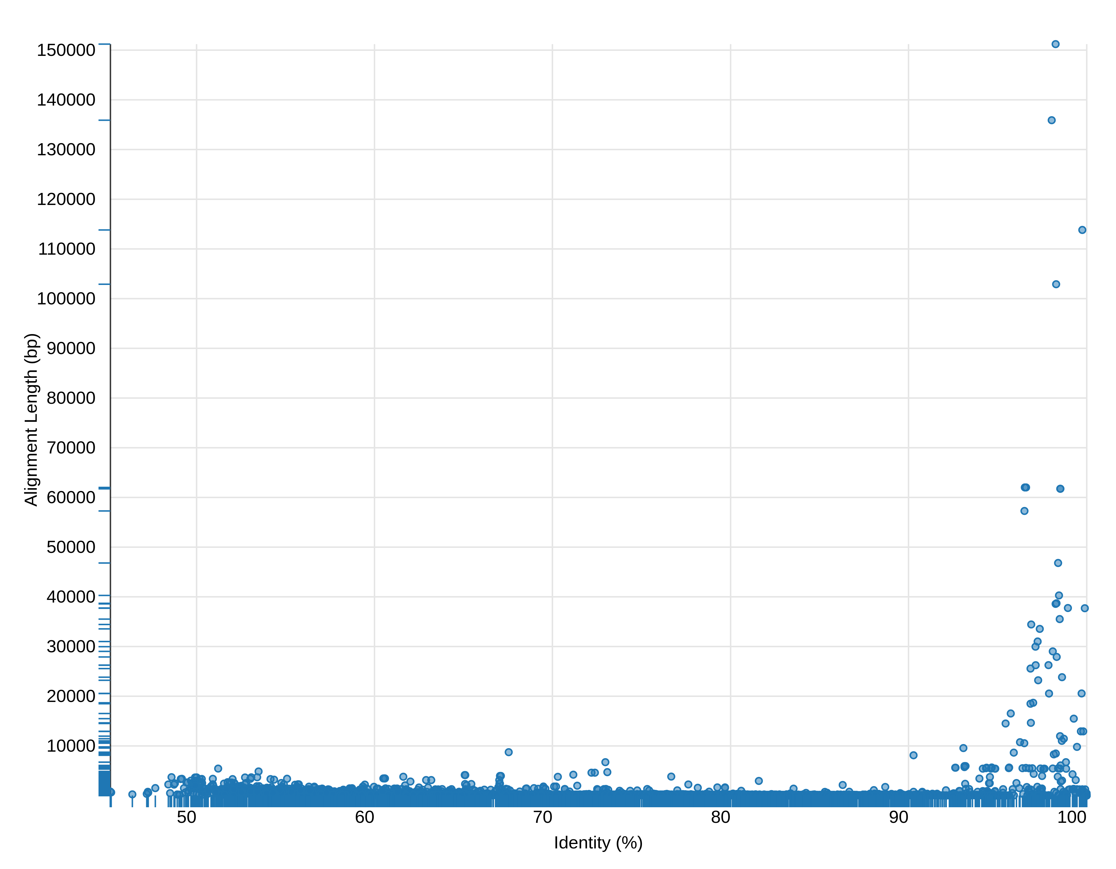 Open image in new tab
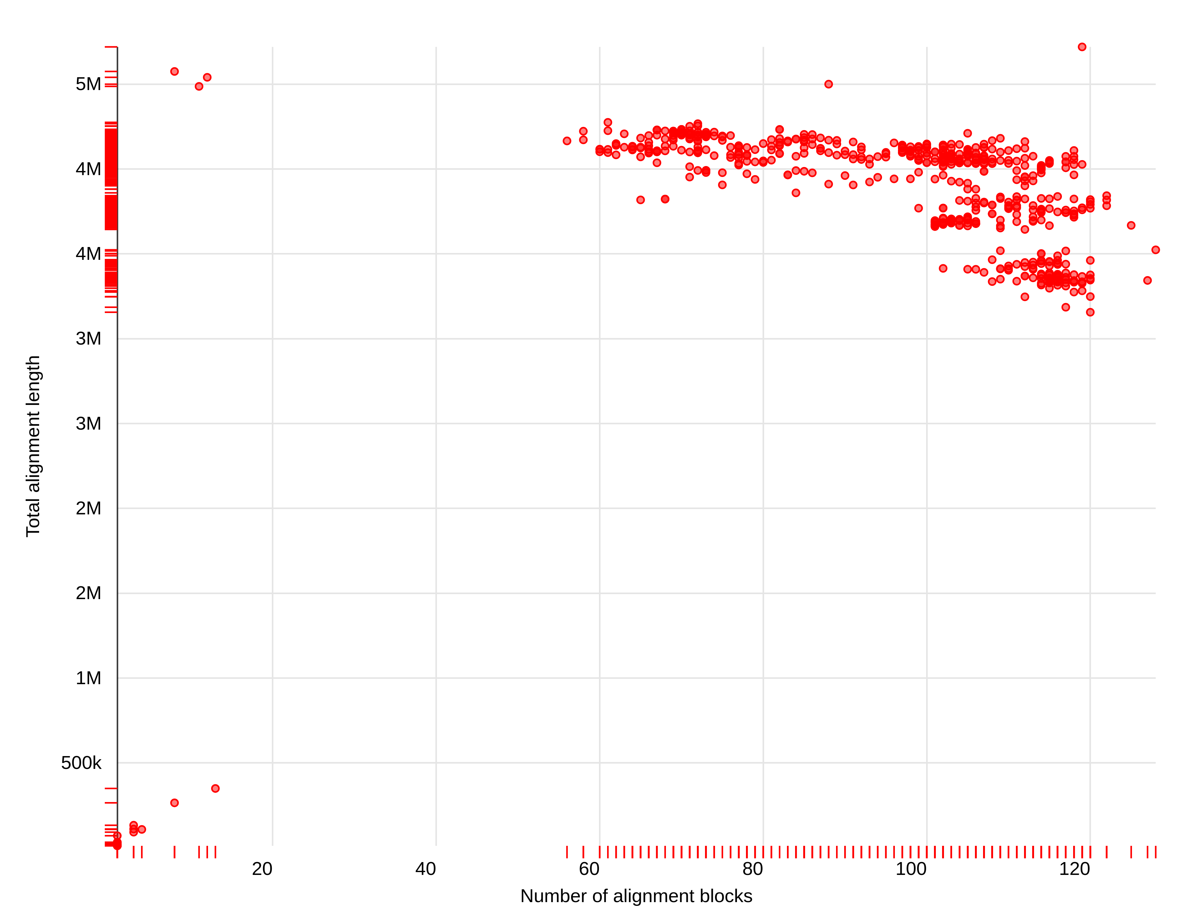 Open image in new tab
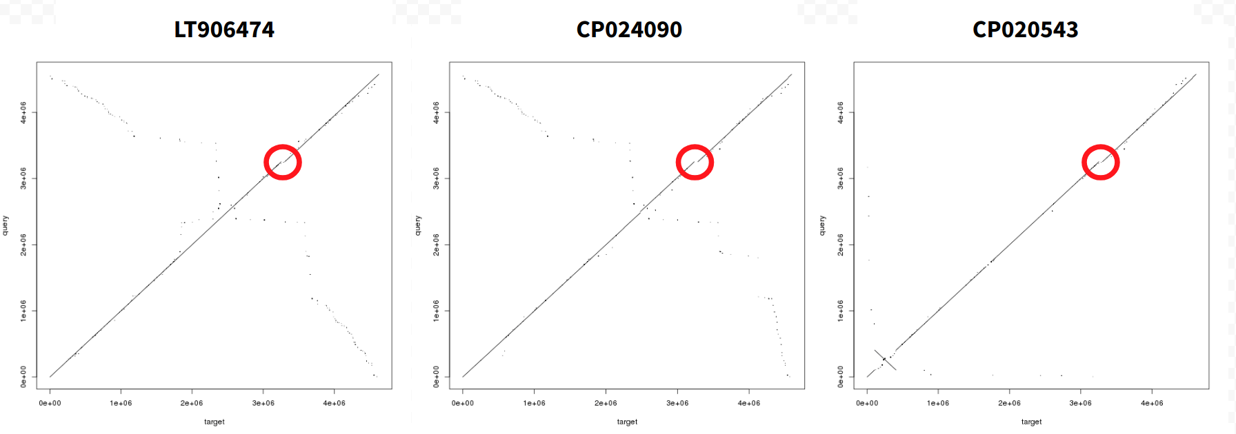 Open image in new tab
Open image in new tab
 Open image in new tab
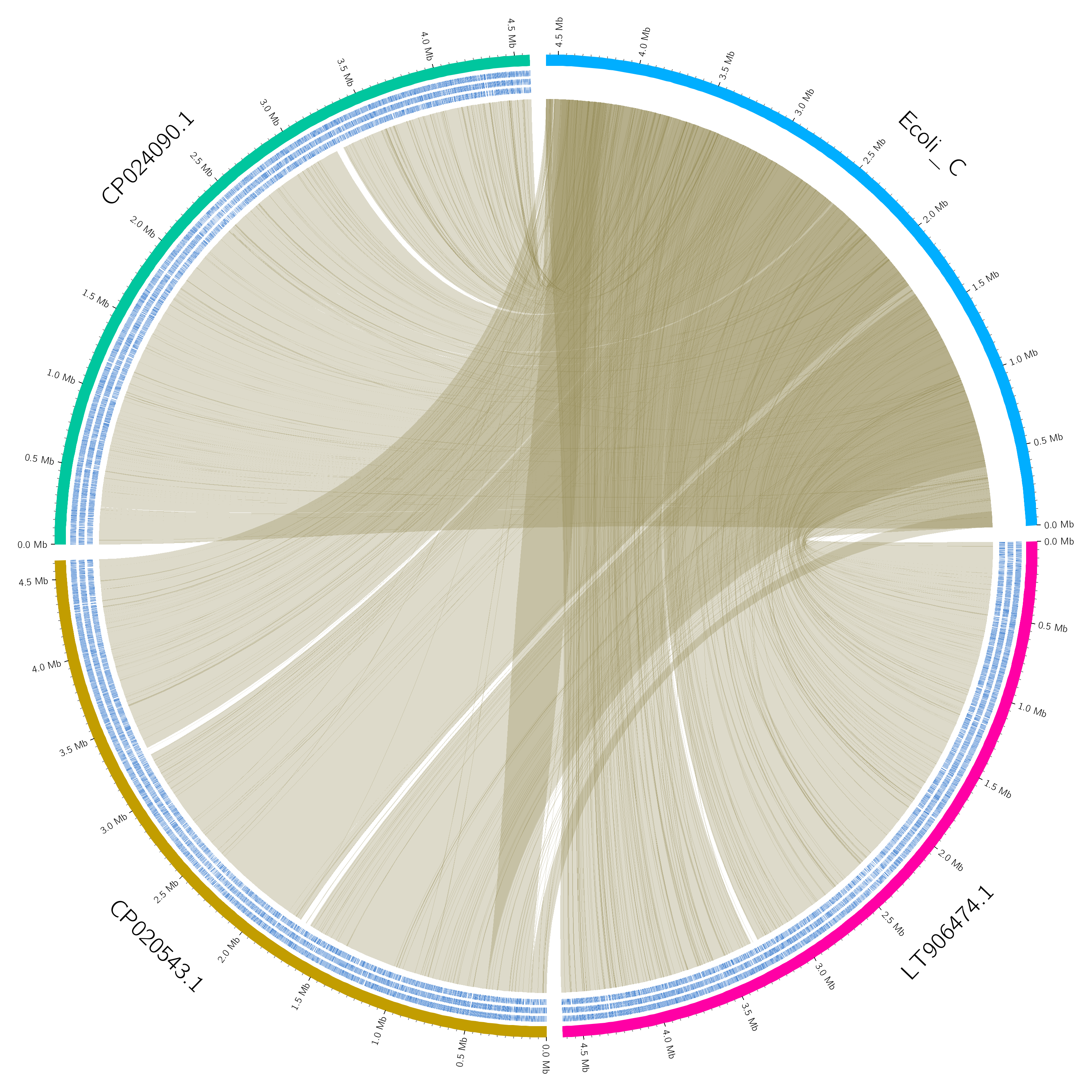 Open image in new tab
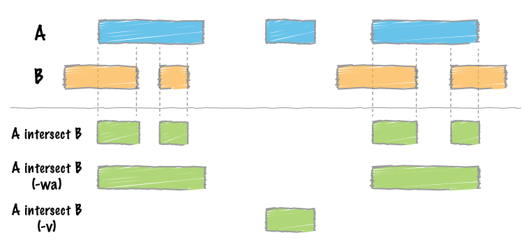 Open image in new tab