Object tracking using CellProfiler
| Author(s) |
|
| Reviewers |
|
OverviewQuestions:
Objectives:
How to segment and track objects in fluorescence time-lapse microscopy images?
Can the same workflow be reused on data from another discipline, such as Earth observation (tracking atmospheric rivers)?
Requirements:
Segment fluorescent objects using CellProfiler in Galaxy
Track objects over multiple frames using CellProfiler in Galaxy
Reuse the same CellProfiler tracking pipeline on an Earth-observation time series (cross-discipline reuse)
- Introduction to Galaxy Analyses
- tutorial Hands-on: FAIR Bioimage Metadata
- tutorial Hands-on: REMBI - Recommended Metadata for Biological Images – metadata guidelines for bioimaging data
- tutorial Hands-on: Creating, Editing and Importing Galaxy Workflows
Time estimation: 1 hourLevel: Intermediate IntermediateSupporting Materials:Published: Mar 17, 2021Last modification: Jun 23, 2026License: Tutorial Content is licensed under Creative Commons Attribution 4.0 International License. The GTN Framework is licensed under MITpurl PURL: https://gxy.io/GTN:T00182rating Rating: 5.0 (0 recent ratings, 1 all time)version Revision: 12
Most biological processes are dynamic and observing them over time can provide valuable insights. Combining fluorescent markers with time-lapse imaging is a common approach to collect data on dynamic cellular processes such as cell division (e.g. Neumann et al. 2010, Hériché et al. 2014). However, automated time-lapse imaging can produce large amounts of data that can be challenging to process. One of these challenges is the tracking of individual objects as it is often impossible to manually follow a large number of objects over many time points.
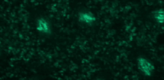
To demonstrate how automatic tracking can be applied in such situations, this tutorial will track dividing nuclei in a short time-lapse recording of one mitosis of a syncytial blastoderm stage Drosophila embryo expressing a GFP-histone gene that labels chromatin.
Tracking is done by first segmenting objects then linking objects between consecutive frames. Linking is done by matching objects and several criteria or matching rules are available. Here we will link objects if they significantly overlap between the current and previous frames.
It is expected that you are already familiar with the Galaxy interface and the workflow editor. If this is not the case, we recommend you to complete the requirements listed at the start of this tutorial.
Warning: Important information: CellProfiler in GalaxyThe Galaxy CellProfiler ( Galaxy version 3.1.9+galaxy0) tool takes two inputs: a CellProfiler pipeline and an image collection. Some pipelines created with stand-alone CellProfiler may not work with the Galaxy CellProfiler tool. Some reasons are:
- The pipeline was built with a different version of CellProfiler. The Galaxy tool currently uses CellProfiler 3.9.
- Modules used by the pipeline aren’t available in Galaxy.
- Parameters for some CellProfiler modules are limited/constrained compared to the stand-alone version, most notably:
- Parameters require manual input from the user whereas, in the stand-alone version, some modules can inherit parameter values from other modules.
- Input and output file locations are set by Galaxy and can’t be set by the user.
- Metadata extraction from file names is limited to a set of fixed patterns.
It is recommended to build a CellProfiler pipeline using the Galaxy interface if the pipeline is to be run by Galaxy.
AgendaIn this tutorial, we will cover:
The same CellProfiler tracking pipeline can be applied to time series from very different scientific domains. This tutorial can be followed with a bioimaging dataset (dividing cell nuclei in a fluorescence microscopy recording) or an Earth-observation dataset (atmospheric rivers in a climate-reanalysis time series). The pipeline is the same in both paths — you build it once, exactly the same way; only the input data and a few names (the object name and the file-name marker) change. Choose the path that interests you most.
Hands-on: Choose Your Own TutorialThis is a 'Choose Your Own Tutorial' (CYOT) section (also known as 'Choose Your Own Analysis' (CYOA)), where you can select between multiple paths. Click one of the buttons below to select how you want to follow the tutorial
Pick a dataset: a fluorescence-microscopy recording of dividing cell nuclei, or a climate-reanalysis time series of atmospheric rivers. You build and run the same CellProfiler pipeline either way.
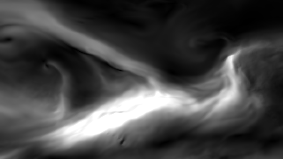
Comment: Tracking atmospheric rivers with a cell-tracking pipelineIn the Earth-observation path we reuse this same CellProfiler object-tracking pipeline — built to follow dividing nuclei — to detect and track atmospheric rivers: long, narrow filaments of intense water-vapour transport in the atmosphere (the “rivers in the sky” that deliver much of the world’s extreme rainfall). This is a cross-discipline experiment from the OSCARS-FIESTA project. Why does it work? An atmospheric river is a bright, elongated filament on a dark background in a map of vertically integrated vapour transport (IVT) — morphologically much like the bright nuclei the pipeline was built for. A river that intensifies, drifts and splits over time is the climate-science analogue of a dividing nucleus, so the same segment-then-link-by-overlap approach tracks it. The preprocessing notebooks, the full Galaxy run provenance, and a citable archive are in the OSCARS-FIESTA example repository.
Get data
This tutorial will use a time-lapse recording of nuclei progressing through mitotic anaphase during early Drosophila embryogenesis. The nuclei are labelled on chromatin with a GFP-histone marker and have been imaged every 7 seconds using a laser scanning confocal microscope with a 40X objective. The images are saved as a zip archive on Zenodo and need to be uploaded to the Galaxy server before they can be used.
 Open image in new tab
Hands On: Data upload — bioimaging
Create a new history for this tutorial. When you log in for the first time, an empty, unnamed history is created by default. You can simply rename it.
To create a new history simply click the new-history icon at the top of the history panel:
- Import galaxy-upload the files from Zenodo or from the shared data library.
- Important: If setting the type to ‘Auto-detect’, make sure that after upload, the datatype is set to zip.
https://doi.org/10.5281/zenodo.4567084/files/drosophila_sample.zip
- Copy the link location
Click galaxy-upload Upload at the top of the activity panel
- Select galaxy-wf-edit Paste/Fetch Data
Paste the link(s) into the text field
Press Start
- Close the window
- Rename galaxy-pencil the file to drosophila_embryo.zip

This path uses a time series of atmospheric-river activity over the North Pacific during an early-February 2017 event. Each frame is a map of the vertically integrated water-vapour transport (IVT) magnitude from the ERA5 climate reanalysis, rendered so that the atmospheric river appears as a bright filament on a dark background — one frame every 6 hours. The frames are saved as a zip archive on Zenodo and need to be uploaded to the Galaxy server before they can be used.
 Open image in new tab
Hands On: Data upload — Earth observation
Create a new history for this tutorial. When you log in for the first time, an empty, unnamed history is created by default. You can simply rename it.
To create a new history simply click the new-history icon at the top of the history panel:
- Import galaxy-upload the atmospheric-river IVT frames from Zenodo.
- Important: If setting the type to ‘Auto-detect’, make sure that after upload, the datatype is set to zip.
https://zenodo.org/records/20813832/files/npacific_ivt_frames.zip
- Copy the link location
Click galaxy-upload Upload at the top of the activity panel
- Select galaxy-wf-edit Paste/Fetch Data
Paste the link(s) into the text field
Press Start
- Close the window
- Rename galaxy-pencil the file to npacific_ivt_frames.zip
Comment: How the atmospheric-river frames were preparedThe frames come from the ERA5 reanalysis Hersbach et al. 2020 accessed through the public, anonymous ARCO-ERA5 archive. For each 6-hourly time step we took the eastward and northward vertically integrated vapour-transport components and combined them into the IVT magnitude, IVT = √(u² + v²), over the North Pacific (2 – 11 February 2017). Each field was rescaled to an 8-bit image (bright river on dark background) and written as a three-channel PNG named
NPacific_IVT_0000.png,NPacific_IVT_0001.png, … so the filename carries the time index — exactly the structure the Metadata step below expects. These frames are archived on Zenodo Fouilloux 2026; the preprocessing notebooks, the full Galaxy run provenance, and a citable software archive are in the OSCARS-FIESTA example repository.
Create a CellProfiler pipeline in Galaxy
In this section, we will build a CellProfiler pipeline from scratch in Galaxy. We need to:
- Read the images and the metadata
- Convert the colour images to grayscale
- Segment the objects (nuclei / atmospheric rivers)
- Extract features from the segmented objects
- Perform tracking
- Produce some useful output files
A pipeline is built by chaining together Galaxy tools representing CellProfiler modules and must start with the Starting modules ( Galaxy version 3.1.9+galaxy1) tool and end with the CellProfiler ( Galaxy version 3.1.9+galaxy0) tool.
- Metadata is needed to tell CellProfiler what a temporal sequence of images is and what the order of images is in the sequence.
- CellProfiler is designed to work primarily with grayscale images. Since we don’t need the colour information, we convert colour images to grayscale type.
- Segmentation means identifying the objects in each image. In CellProfiler, this is done by thresholding the intensity level in each image.
- When we perform tracking we’re usually interested in quantifying how some properties of the objects evolve over time. Also, sometimes we may want to do tracking by matching objects based on some property of the objects (e.g. a shape measurement). Therefore, for each segmented object, we compute some features, i.e. numerical descriptors of some properties of the object.
- Tracking will provide the information required to allow downstream data analysis tools to link the features into a multidimensional time series.
The pipeline you build is the same for both paths. Only two pieces of text differ, depending on which dataset you chose:
Comment: Names to use in the bioimaging path
- The file-name marker used to recognise and order the images is
GFPHistone.- The object name we give the segmented objects is
Nuclei(and the tracked image isTrackedNuclei).
Comment: Names to use in the Earth-observation path
- The file-name marker used to recognise and order the images is
IVT.- The object name we give the segmented objects is
Rivers(and the tracked image isTrackedRivers).
Create a new workflow
Hands On: Creating a new workflow
Create a new workflow
- Click Workflow on the top bar
- Click the new workflow galaxy-wf-new button
- Give it a clear and memorable name
- Clicking Save will take you directly into the workflow editor for that workflow
- Need more help? Please see the How to make a workflow subsection here
The next steps will add new tools using the workflow editor. Remember to save the workflow when done (or anytime) to not lose your input parameters.
Read the images
Hands On: Reading images
Add Inputs → Input Dataset to the workflow
Add tool Unzip with the following parameter:
- param-select “Extract single file”:
All files
Get the metadata
CommentThe Starting modules tool combines four CellProfiler modules that are always used together at the start of a pipeline. These modules are:
- Images
- Metadata
- NamesAndTypes
- Groups
Hands On: Getting metadata — bioimaging
Starting modules ( Galaxy version 3.1.9+galaxy1) with the following parameters:
- Images
- “Do you want to filter only the images?”:
Select the images only- Metadata
“Do you want to extract the metadata?”:
Yes, specify metadata
- param-repeat Insert new metadata
- “Metadata extraction method”:
Extract from file/folder names- “Metadata source”:
File name- “Select the pattern to extract metadata from the file name”:
field1_field2_field3“Extract metadata from”:
Images matching a rule
- “Match the following rules”:
All- param-repeat Insert filtering rules:
- “Select the filtering criteria”:
File- "”operator:
Does- “contain”:
Contain regular expression- “match_value”:
GFPHistone- NamesAndTypes
- “Process 3D”:
No, do not process 3D data- “Assign a name to”:
Give images one of several names depending on the metadata
- param-repeat Insert another image:
- “Match the following rules”:
Allparam-repeat Insert rule:
“Select rule criteria”:
File
- “operator”:
Does- “contain”:
Contain regular expression- “match_value”:
GFPHistone- “Select the image type”:
Color image- “Name to assign these images”:
OrigColor- “Set intensity range from”:
Image metadata- “Image matching method”:
Metadata- Groups
- “Do you want to group your images?”:
Yes, group the images- “Metadata category”:
field1
QuestionHow are we capturing metadata and what type of metadata are we getting?
Metadata is obtained from the filenames by extracting three text fields separated by an underscore. The metadata we get is “DrosophilaEmbryo”, “GFPHistone” and numbers with leading zeros. These three fields represent respectively the sample identifier, the marker visualized in the image and the index in the time series.
Hands On: Getting metadata — Earth observation
Starting modules ( Galaxy version 3.1.9+galaxy1) with the following parameters:
- Images
- “Do you want to filter only the images?”:
Select the images only- Metadata
“Do you want to extract the metadata?”:
Yes, specify metadata
- param-repeat Insert new metadata
- “Metadata extraction method”:
Extract from file/folder names- “Metadata source”:
File name- “Select the pattern to extract metadata from the file name”:
field1_field2_field3“Extract metadata from”:
Images matching a rule
- “Match the following rules”:
All- param-repeat Insert filtering rules:
- “Select the filtering criteria”:
File- "”operator:
Does- “contain”:
Contain regular expression- “match_value”:
IVT- NamesAndTypes
- “Process 3D”:
No, do not process 3D data- “Assign a name to”:
Give images one of several names depending on the metadata
- param-repeat Insert another image:
- “Match the following rules”:
Allparam-repeat Insert rule:
“Select rule criteria”:
File
- “operator”:
Does- “contain”:
Contain regular expression- “match_value”:
IVT- “Select the image type”:
Color image- “Name to assign these images”:
OrigColor- “Set intensity range from”:
Image metadata- “Image matching method”:
Metadata- Groups
- “Do you want to group your images?”:
Yes, group the images- “Metadata category”:
field1
QuestionHow are we capturing metadata and what type of metadata are we getting?
Metadata is obtained from the filenames by extracting three text fields separated by an underscore. The metadata we get is “NPacific”, “IVT” and numbers with leading zeros. These three fields represent respectively the region identifier, the variable visualized in the image (the integrated vapour transport) and the index in the time series.
QuestionHow will CellProfiler form a temporal sequence?
Images will be grouped based on field1 which here is the sample/region identifier and ordered alpha-numerically (by default) which will order them by field3 (the time series index) since fields 1 and 2 are constant.
Convert the images to grayscale
Hands On: Colour to grayscale conversion
- ColorToGray ( Galaxy version 3.1.9+galaxy0) with the following parameters:
- “Select the input CellProfiler pipeline”: Connect output of Starting Modules tool to input of ColorToGray
- “Enter the name of the input image”:
OrigColor- “Conversion method”:
Combine
- “Name the output image”:
OrigGray- “Image type”:
RGB
- “Relative weight of the red channel”:
1- “Relative weight of the green channel”:
1- “Relative weight of the blue channel”:
1
Segmentation
The first step to track objects starts with the identification of those objects on the images.
Hands On: Nuclei segmentation
- IdentifyPrimaryObjects ( Galaxy version 3.1.9+galaxy1) with the following parameters:
- param-file “Select the input CellProfiler pipeline”: output of ColorToGray tool
- “Use advanced settings?”:
Yes, use advanced settings
- “Enter the name of the input image (from NamesAndTypes)”:
OrigGray- “Enter the name of the primary objects to be identified”:
Nuclei- “Typical minimum diameter of objects, in pixel units (Min)”:
30- “Typical maximum diameter of objects, in pixel units (Max)”:
9999- “Discard objects outside diameter range?”:
Yes- “Discard objects touching the border of the image?”:
Yes- “Threshold strategy”:
Global
- “Thresholding method”:
Otsu
- “Two-class or three-class thresholding?”:
Three classes
- “Assign pixels in the middle intensity class to the foreground or the background?”:
Background- Threshold smoothing scale”:
1.3488- Threshold correction factor”:
1- Lower bound on threshold”:
0.01- Upper bound on threshold”:
1- “Method to distinguish clumped objects”:
Intensity
- “Method to draw dividing lines between clumped objects”:
Intensity
- “Automatically calculate size of smoothing filter for declumping?”:
Yes- “Automatically calculate minimum allowed distance between local maxima?”:
Yes- “Speed up by using lower-resolution mage to find local maxima?”:
Yes- “Fill holes in identified objects”:
After both thresholding and declumping- “Handling of objects if excessive number of objects identified”:
Continue
Hands On: Atmospheric-river segmentation
- IdentifyPrimaryObjects ( Galaxy version 3.1.9+galaxy1) with the following parameters:
- param-file “Select the input CellProfiler pipeline”: output of ColorToGray tool
- “Use advanced settings?”:
Yes, use advanced settings
- “Enter the name of the input image (from NamesAndTypes)”:
OrigGray- “Enter the name of the primary objects to be identified”:
Rivers- “Typical minimum diameter of objects, in pixel units (Min)”:
30- “Typical maximum diameter of objects, in pixel units (Max)”:
9999- “Discard objects outside diameter range?”:
Yes- “Discard objects touching the border of the image?”:
Yes- “Threshold strategy”:
Global
- “Thresholding method”:
Otsu
- “Two-class or three-class thresholding?”:
Three classes
- “Assign pixels in the middle intensity class to the foreground or the background?”:
Background- Threshold smoothing scale”:
1.3488- Threshold correction factor”:
1- Lower bound on threshold”:
0.01- Upper bound on threshold”:
1- “Method to distinguish clumped objects”:
Intensity
- “Method to draw dividing lines between clumped objects”:
Intensity
- “Automatically calculate size of smoothing filter for declumping?”:
Yes- “Automatically calculate minimum allowed distance between local maxima?”:
Yes- “Speed up by using lower-resolution mage to find local maxima?”:
Yes- “Fill holes in identified objects”:
After both thresholding and declumping- “Handling of objects if excessive number of objects identified”:
Continue
Feature extraction
Once the objects of interest are identified, we extract features, i.e. numerical descriptors of object properties. We do this because we may be interested in analysing the evolution of these properties over time or want to use them in the tracking procedure to match objects over time.
Hands On: Shape features
- MeasureObjectSizeShape ( Galaxy version 3.1.9+galaxy0) with the following parameters:
- param-file “Select the input CellProfiler pipeline”: output of IdentifyPrimaryObjects tool
- In “new object”:
- param-repeat “Insert new object”
- “Enter the name of the object to measure”:
Nuclei- “Calculate the Zernike features?”:
No
Hands On: Intensity features
- MeasureObjectIntensity ( Galaxy version 3.1.9+galaxy0) with the following parameters:
- param-file “Select the input CellProfiler pipeline”: output of MeasureObjectSizeShape tool
- In “new image”:
- param-repeat “Insert new image”
- “Enter the name of an image to measure”:
OrigGray- In “new object”:
- param-repeat “Insert new object”
- “Enter the name of the objects to measure”:
Nuclei
Hands On: Shape features
- MeasureObjectSizeShape ( Galaxy version 3.1.9+galaxy0) with the following parameters:
- param-file “Select the input CellProfiler pipeline”: output of IdentifyPrimaryObjects tool
- In “new object”:
- param-repeat “Insert new object”
- “Enter the name of the object to measure”:
Rivers- “Calculate the Zernike features?”:
No
Hands On: Intensity features
- MeasureObjectIntensity ( Galaxy version 3.1.9+galaxy0) with the following parameters:
- param-file “Select the input CellProfiler pipeline”: output of MeasureObjectSizeShape tool
- In “new image”:
- param-repeat “Insert new image”
- “Enter the name of an image to measure”:
OrigGray- In “new object”:
- param-repeat “Insert new object”
- “Enter the name of the objects to measure”:
Rivers
Track the objects
With the objects and the relevant features measured, we are now ready to start the tracking step!
Hands On: Object tracking
- TrackObjects ( Galaxy version 3.1.9+galaxy0) with the following parameters:
- param-file “Select the input CellProfiler pipeline”: output of MeasureObjectIntensity tool
- “Enter the name of the objects to track”:
Nuclei- “Choose a tracking method”:
Overlap
- “Maximum pixel distance to consider matches”:
50- “Filter objects by lifetime?”:
No- “Select display option?”:
Color and Number- “Save color-coded image?”:
Yes
- “Name the output image”:
TrackedNuclei
Hands On: Object tracking
- TrackObjects ( Galaxy version 3.1.9+galaxy0) with the following parameters:
- param-file “Select the input CellProfiler pipeline”: output of MeasureObjectIntensity tool
- “Enter the name of the objects to track”:
Rivers- “Choose a tracking method”:
Overlap
- “Maximum pixel distance to consider matches”:
50- “Filter objects by lifetime?”:
No- “Select display option?”:
Color and Number- “Save color-coded image?”:
Yes
- “Name the output image”:
TrackedRivers
Visualize results
To make sure that the tracking has gone as expected, we will have a look at the original images together with the results of the segmentation step. And we will visualize them together (in tiles) for easier comparison.
Hands On: Visualize segmentation outcome
- OverlayOutlines ( Galaxy version 3.1.9+galaxy0) with the following parameters:
- param-file “Select the input CellProfiler pipeline”: output of TrackObjects tool
- “Display outlines on a blank image?”:
No
- “Enter the name of image on which to display outlines”:
OrigGray- “Outline display mode”:
Color
- In “Outline”:
- param-repeat “Insert Outline”
- “Enter the name of the objects to display”:
Nuclei- “Select outline color”: (red)
- “Name the output image”:
OutlineImage- “How to outline”:
Inner
Hands On: Tiling images
- Tile ( Galaxy version 3.1.9+galaxy0) with the following parameters:
- param-file “Select the input CellProfiler pipeline”: output of OverlayOutlines tool
- “Enter the name of an input image”:
OrigColor- “Name the output image”:
TiledImages- “Tile assembly method”:
Within cycles
- “Automatically calculate number of rows?”:
No
- “Final number of rows”:
1- “Automatically calculate number of columns?”:
Yes- “Image corner to begin tiling”:
top left- “Direction to begin tiling”:
row- “Use meander mode?”:
No- In “Another image”:
- param-repeat “Insert Another image”
- “Enter the name of an additional image to tile”:
OutlineImage- param-repeat “Insert Another image”
- “Enter the name of an additional image to tile”:
TrackedNuclei
Hands On: Visualize segmentation outcome
- OverlayOutlines ( Galaxy version 3.1.9+galaxy0) with the following parameters:
- param-file “Select the input CellProfiler pipeline”: output of TrackObjects tool
- “Display outlines on a blank image?”:
No
- “Enter the name of image on which to display outlines”:
OrigGray- “Outline display mode”:
Color
- In “Outline”:
- param-repeat “Insert Outline”
- “Enter the name of the objects to display”:
Rivers- “Select outline color”: (red)
- “Name the output image”:
OutlineImage- “How to outline”:
Inner
Hands On: Tiling images
- Tile ( Galaxy version 3.1.9+galaxy0) with the following parameters:
- param-file “Select the input CellProfiler pipeline”: output of OverlayOutlines tool
- “Enter the name of an input image”:
OrigColor- “Name the output image”:
TiledImages- “Tile assembly method”:
Within cycles
- “Automatically calculate number of rows?”:
No
- “Final number of rows”:
1- “Automatically calculate number of columns?”:
Yes- “Image corner to begin tiling”:
top left- “Direction to begin tiling”:
row- “Use meander mode?”:
No- In “Another image”:
- param-repeat “Insert Another image”
- “Enter the name of an additional image to tile”:
OutlineImage- param-repeat “Insert Another image”
- “Enter the name of an additional image to tile”:
TrackedRivers
Save the images and features
The tiled images and the features computed in previous steps are now exported to the Galaxy history ready to be analyzed.
Hands On: Save the images
- SaveImages ( Galaxy version 3.1.9+galaxy1) with the following parameters:
- param-file “Select the input CellProfiler pipeline”: output of Tile tool
- “Select the type of image to save”:
Image
- “Saved the format to save the image(s)”:
png- “Enter the name of the image to save”:
TiledImages- “Select method for constructing file names”:
From image filename
- “Enter the image file name”:
OrigColor- “Append a suffix to the image file name”:
Yes
- “Text to append to the image file name”:
_tile- “Overwrite existing files without warning?”:
Yes- “When to save”:
Every cycle- “Record the file and path information to the saved image?”:
No
Hands On: Export tabular data to character-delimited text files
- ExportToSpreadsheet ( Galaxy version 3.1.9+galaxy1) with the following parameters:
- param-file “Select the input CellProfiler pipeline”: output of SaveImages tool
- “Select the column delimiter”:
Comma (",")- “Add a prefix to file names?”:
Do not add prefix to the file name- “Overwrite existing files without warning”:
Yes- “Add image metadata columns to your object data file”:
Yes- “Representation of Nan/Inf”:
NaN- “Calculate the per-image mean values for object measurements?”:
Yes- “Calculate the per-image median values for object measurements?”:
Yes- “Calculate the per-image standard deviation values for object measurements?”:
Yes- “Create a GenePattern GCT file?”:
NoCommentBy default all measurement types are exported. This is in contrast to the stand-alone version of CellProfiler which allows choosing which measurement types to save.
Run the pipeline with CellProfiler
As mentioned in the introduction, the tool CellProfiler ( Galaxy version 3.1.9+galaxy0) takes as input the pipeline that we have been assembling over this tutorial and the input data. We are now ready to finally run CellProfiler!
Hands On: Running the pipeline with CellProfiler
- CellProfiler ( Galaxy version 3.1.9+galaxy0) with the following parameters:
- param-file “Pipeline file”: `output of ExportToSpreadsheet tool
- “Are the input images packed into a tar archive?”:
No
- param-collection “Images”: output of Unzip tool
- “Detailed logging file?”:
YesRun the workflow.
- Click on Workflows on the Activity Bar on the left.
- At the top of the resulting page you will have the option to switch between the My workflows, Workflows shared with me and Public workflows tabs.
- Select the tab you want to see all workflows in that category
Search for your desired workflow.
- Click on the workflow name: a pop-up window opens with a preview of the workflow.
- To run it directly: click Run (top-right).
- Recommended: click Import (left of Run) to make your own local copy under Workflows / My Workflows.
CommentIf the pipeline fails, inspect the CellProfiler log file for clues about errors. A common source of errors is not providing the correct information to a module such as pointing a CellProfiler module at a non-existent dataset (e.g. with a typo in the name).
QuestionHow many nuclei have been tracked?
Five objects were detected but only four of these were nuclei.
QuestionHow could we get rid of tracks that don’t correspond to nuclei?
Objects that are not nuclei appear to be transient so one solution would be to require the tracks to have a minimal length. This can be done using the “Filter objects by lifetime” parameter of the TrackObjects module.
QuestionWhere is the data needed to plot change in nuclei eccentricity over time?
The data is in the csv file called Nuclei in the CellProfiler pipeline output data set.
The pipeline outlines the atmospheric-river filaments and links them across the 6-hourly frames, assigning each a track number — exactly as it links dividing nuclei across microscopy frames.
QuestionWhere is the data needed to plot how an atmospheric river’s length changes over time?
The data is in the csv file called Rivers in the CellProfiler pipeline output data set: each row is one river in one frame, with its shape measurements (e.g. major axis length) and its TrackObjects label, so you can follow a single track over time.
Comment: Is this a scientifically valid atmospheric-river tracker?This tutorial shows that the method transfers: the same segment-then-link-by-overlap pipeline detects and tracks atmospheric rivers. It uses CellProfiler’s generic intensity thresholding, not the established meteorological criteria Guan and Waliser 2015 (e.g. an IVT threshold plus a length > 2000 km and length-to-width > 2 geometry test). In the OSCARS-FIESTA study, the same overlap-tracking approach with those criteria applied recovered five distinct atmospheric-river tracks over this ten-day window and followed one persistent river for about five and a half days. That repository (with a citable archive and a full provenance trail) is the place to go for a quantitative atmospheric-river analysis.
Conclusion
We’ve run a CellProfiler pipeline on Galaxy to segment and track objects in a time series, exported images to visually inspect the outcome, and saved tables of computed object features in comma-separated text files for future analysis.
You also saw that the same pipeline can be applied to data from a completely different discipline: a pipeline built to track dividing nuclei in fluorescence microscopy was reused — only its object name and file-name marker retargeted — to detect and track atmospheric rivers in a climate-reanalysis time series. A “bright objects that move, merge and split on a dark background” problem looks the same to CellProfiler whether the objects are nuclei under a microscope or rivers of water vapour seen from space. This kind of cross-discipline reuse is exactly what FAIR, well-described Galaxy workflows make possible.
You've Finished the Tutorial
Key points
CellProfiler in Galaxy can be used to track objects in time-lapse microscopy images
The same Galaxy CellProfiler pipeline can track objects across scientific domains — here a nucleus-tracking pipeline is reused, with only its parameters retargeted, to track atmospheric rivers in climate reanalysis data
Frequently Asked Questions
Have questions about this tutorial? Have a look at the available FAQ pages and support channelsUseful literature
Further information, including links to documentation and original publications, regarding the tools, analysis techniques and the interpretation of results described in this tutorial can be found here.
References
- Neumann, B., T. Walter, J.-K. Hériché, J. Bulkescher, H. Erfle et al., 2010 Phenotypic profiling of the human genome by time-lapse microscopy reveals cell division genes. Nature 464: 721–727. 10.1038/nature08869
- Hériché, J.-K., J. G. Lees, I. Morilla, T. Walter, B. Petrova et al., 2014 Integration of biological data by kernels on graph nodes allows prediction of new genes involved in mitotic chromosome condensation (D. G. Drubin, Ed.). Molecular Biology of the Cell 25: 2522–2536. 10.1091/mbc.e13-04-0221
- Guan, B., and D. E. Waliser, 2015 Detection of atmospheric rivers: Evaluation and application of an algorithm for global studies. Journal of Geophysical Research: Atmospheres 120: 12514–12535. 10.1002/2015JD024257
- Hersbach, H., B. Bell, P. Berrisford, S. Hirahara, A. Horányi et al., 2020 The ERA5 global reanalysis. Quarterly Journal of the Royal Meteorological Society 146: 1999–2049. 10.1002/qj.3803
- Fouilloux, A., 2026 Atmospheric-river IVT frames (North Pacific, Feb 2017) – Galaxy CellProfiler object-tracking tutorial data. Data set. 10.5281/zenodo.20813831
Feedback
Did you use this material as an instructor? Feel free to give us feedback on how it went.
Did you use this material as a learner or student? Click the form below to leave feedback.

Citing this Tutorial
- Yi Sun, Beatriz Serrano-Solano, Jean-Karim Hériché, Anne Fouilloux, Object tracking using CellProfiler (Galaxy Training Materials). https://training.galaxyproject.org/training-material/topics/imaging/tutorials/object-tracking-using-cell-profiler/tutorial.html Online; accessed TODAY
- Hiltemann, Saskia, Rasche, Helena et al., 2023 Galaxy Training: A Powerful Framework for Teaching! PLOS Computational Biology 10.1371/journal.pcbi.1010752
- Batut et al., 2018 Community-Driven Data Analysis Training for Biology Cell Systems 10.1016/j.cels.2018.05.012
@misc{imaging-object-tracking-using-cell-profiler,
author = "Yi Sun and Beatriz Serrano-Solano and Jean-Karim Hériché and Anne Fouilloux",
	title = "Object tracking using CellProfiler (Galaxy Training Materials)",
	year = "",
	month = "",
	day = "",
	url = "\url{https://training.galaxyproject.org/training-material/topics/imaging/tutorials/object-tracking-using-cell-profiler/tutorial.html}",
	note = "[Online; accessed TODAY]"
}
@article{Hiltemann_2023,
	doi = {10.1371/journal.pcbi.1010752},
	url = {https://doi.org/10.1371%2Fjournal.pcbi.1010752},
	year = 2023,
	month = {jan},
	publisher = {Public Library of Science ({PLoS})},
	volume = {19},
	number = {1},
	pages = {e1010752},
	author = {Saskia Hiltemann and Helena Rasche and Simon Gladman and Hans-Rudolf Hotz and Delphine Larivi{\`{e}}re and Daniel Blankenberg and Pratik D. Jagtap and Thomas Wollmann and Anthony Bretaudeau and Nadia Gou{\'{e}} and Timothy J. Griffin and Coline Royaux and Yvan Le Bras and Subina Mehta and Anna Syme and Frederik Coppens and Bert Droesbeke and Nicola Soranzo and Wendi Bacon and Fotis Psomopoulos and Crist{\'{o}}bal Gallardo-Alba and John Davis and Melanie Christine Föll and Matthias Fahrner and Maria A. Doyle and Beatriz Serrano-Solano and Anne Claire Fouilloux and Peter van Heusden and Wolfgang Maier and Dave Clements and Florian Heyl and Björn Grüning and B{\'{e}}r{\'{e}}nice Batut and},
	editor = {Francis Ouellette},
	title = {Galaxy Training: A powerful framework for teaching!},
	journal = {PLoS Comput Biol}
}
Funding
These individuals or organisations provided funding support for the development of this resource
Congratulations on successfully completing this tutorial!You can use Ephemeris's
shed-tools installcommand to install the tools used in this tutorial.shed-tools install [-g GALAXY] [-a API_KEY] -t <(curl https://training.galaxyproject.org/training-material/api/topics/imaging/tutorials/object-tracking-using-cell-profiler/tutorial.json | jq .admin_install_yaml -r)Alternatively you can copy and paste the following YAML
---
install_tool_dependencies: true
install_repository_dependencies: true
install_resolver_dependencies: true
tools:
- name: cp_cellprofiler
  owner: bgruening
  revisions: 0e4dccaafef5
  tool_panel_section_label: Imaging
  tool_shed_url: https://toolshed.g2.bx.psu.edu/
- name: cp_color_to_gray
  owner: bgruening
  revisions: e8f822eeb9fd
  tool_panel_section_label: Imaging
  tool_shed_url: https://toolshed.g2.bx.psu.edu/
- name: cp_common
  owner: bgruening
  revisions: 670975e92458
  tool_panel_section_label: Imaging
  tool_shed_url: https://toolshed.g2.bx.psu.edu/
- name: cp_export_to_spreadsheet
  owner: bgruening
  revisions: d0178bdcd00e
  tool_panel_section_label: Imaging
  tool_shed_url: https://toolshed.g2.bx.psu.edu/
- name: cp_identify_primary_objects
  owner: bgruening
  revisions: b6eec6087271
  tool_panel_section_label: Imaging
  tool_shed_url: https://toolshed.g2.bx.psu.edu/
- name: cp_measure_object_intensity
  owner: bgruening
  revisions: 407925835dd9
  tool_panel_section_label: Imaging
  tool_shed_url: https://toolshed.g2.bx.psu.edu/
- name: cp_measure_object_size_shape
  owner: bgruening
  revisions: acf3aa487283
  tool_panel_section_label: Imaging
  tool_shed_url: https://toolshed.g2.bx.psu.edu/
- name: cp_overlay_outlines
  owner: bgruening
  revisions: 91560258e972
  tool_panel_section_label: Imaging
  tool_shed_url: https://toolshed.g2.bx.psu.edu/
- name: cp_save_images
  owner: bgruening
  revisions: 33f4fa1413fb
  tool_panel_section_label: Imaging
  tool_shed_url: https://toolshed.g2.bx.psu.edu/
- name: cp_tile
  owner: bgruening
  revisions: 443638c10c61
  tool_panel_section_label: Imaging
  tool_shed_url: https://toolshed.g2.bx.psu.edu/
- name: cp_track_objects
  owner: bgruening
  revisions: 1fd453cd757b
  tool_panel_section_label: Imaging
  tool_shed_url: https://toolshed.g2.bx.psu.edu/
- name: unzip
  owner: imgteam
  revisions: 38eec75fbe9b
  tool_panel_section_label: Collection Operations
  tool_shed_url: https://toolshed.g2.bx.psu.edu/