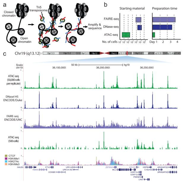
In many eukaryotic organisms, such as humans, the genome is tightly packed and organized with the help of nucleosomes (chromatin). A nucleosome is a complex formed by eight histone proteins that is wrapped with ~147bp of DNA. When the DNA is being actively transcribed into RNA, the DNA will be opened and loosened from the nucleosome complex. Many factors, such as the chromatin structure, the position of the nucleosomes, and histone modifications, play an important role in the organization and accessibility of the DNA. Consequently, these factors are also important for the activation and inactivation of genes. Assay for Transposase-Accessible Chromatin using sequencing (ATAC-Seq) is a method to investigate the accessibility of chromatin and thus a method to determine regulatory mechanisms of gene expression. The method can help identify promoter regions and potential enhancers and silencers. A promoter is the DNA region close to the transcription start site (TSS). It contains binding sites for transcription factors that will recruit the RNA polymerase. An enhancer is a DNA region that can be located up to 1 Mb downstream or upstream of the promoter. When transcription factors bind an enhancer and contact a promoter region, the transcription of the gene is increased. In contrast, a silencer decreases or inhibits the gene’s expression. ATAC-Seq has become popular for identifying accessible regions of the genome as it’s easier, faster and requires less cells than alternative techniques, such as FAIRE-Seq and DNase-Seq.
With ATAC-Seq, to find accessible (open) chromatin regions, the genome is treated with a hyperactive derivative of the Tn5 transposase. A transposase can bind to a transposable element, which is a DNA sequence that can change its position (jump) within a genome (read the two links to get a deeper insight). During ATAC-Seq, the modified Tn5 inserts DNA sequences corresponding to truncated Nextera adapters into open regions of the genome and concurrently, the DNA is sheared by the transposase activity. The read library is then prepared for sequencing, including PCR amplification with full Nextera adapters and purification steps. Paired-end reads are recommended for ATAC-Seq for the reasons described in their guidelines.
In this tutorial we will use data from the study of Buenrostro et al. 2013, the first paper on the ATAC-Seq method. The data is from a human cell line of purified CD4+ T cells, called GM12878. The original dataset had 2 x 200 million reads and would be too big to process in a training session, so we downsampled the original dataset to 200,000 randomly selected reads. We also added about 200,000 reads pairs that will map to chromosome 22 to have a good profile on this chromosome, similar to what you might get with a typical ATAC-Seq sample (2 x 20 million reads in original FASTQ). Furthermore, we want to compare the predicted open chromatin regions to the known binding sites of CTCF, a DNA-binding protein implicated in 3D structure: CTCF. CTCF is known to bind to thousands of sites in the genome and thus it can be used as a positive control for assessing if the ATAC-Seq experiment is good quality. Good ATAC-Seq data would have accessible regions both within and outside of TSS, for example, at some CTCF binding sites. For that reason, we will download binding sites of CTCF identified by ChIP in the same cell line from ENCODE (ENCSR000AKB, dataset ENCFF933NTR).
When working with real data
When you use your own data we suggest you to use this workflow which includes the same steps but is compatible with replicates. If you do not have any control data you can import and edit this workflow, removing all steps with the controls. Controls for the ATAC-Seq procedure are not commonly performed, as discussed in the guidelines, but could be ATAC-Seq of purified DNA.
Your results may be slightly different from the ones presented in this tutorial due to differing versions of tools, reference data, external databases, or because of stochastic processes in the algorithms.
Preprocessing
Get Data
We first need to download the sequenced reads (FASTQs) as well as other annotation files. Then, to increase the number of reads that will map to the reference genome (here human genome version 38, GRCh38/hg38), we need to preprocess the reads.
Hands On: Data upload
Create a new history for this tutorial
To create a new history simply click the new-history icon at the top of the history panel:
Import the files from Zenodo or from
the shared data library (GTN - Material -> epigenetics
-> ATAC-Seq data analysis):
Click galaxy-uploadUpload at the top of the activity panel
Select galaxy-wf-editPaste/Fetch Data
Paste the link(s) into the text field
Press Start
Close the window
As an alternative to uploading the data from a URL or your computer, the files may also have been made available from a shared data library:
Go into Libraries (left panel)
Navigate to the correct folder as indicated by your instructor.
On most Galaxies tutorial data will be provided in a folder named GTN - Material –> Topic Name -> Tutorial Name.
Select the desired files
Click on Add to Historygalaxy-dropdown near the top and select as Datasets from the dropdown menu
In the pop-up window, choose
“Select history”: the history you want to import the data to (or create a new one)
Click on Import
Add a tag called #SRR891268_R1 to the R1 file and a tag called #SRR891268_R2 to the R2 file.
Datasets can be tagged. This simplifies the tracking of datasets across the Galaxy interface. Tags can contain any combination of letters or numbers but cannot contain spaces.
To tag a dataset:
Click on the dataset to expand it
Click on Add Tagsgalaxy-tags
Add tag text. Tags starting with # will be automatically propagated to the outputs of tools using this dataset (see below).
Press Enter
Check that the tag appears below the dataset name
Tags beginning with # are special!
They are called Name tags. The unique feature of these tags is that they propagate: if a dataset is labelled with a name tag, all derivatives (children) of this dataset will automatically inherit this tag (see below). The figure below explains why this is so useful. Consider the following analysis (numbers in parenthesis correspond to dataset numbers in the figure below):
a set of forward and reverse reads (datasets 1 and 2) is mapped against a reference using Bowtie2 generating dataset 3;
dataset 3 is used to calculate read coverage using BedTools Genome Coverageseparately for + and - strands. This generates two datasets (4 and 5 for plus and minus, respectively);
datasets 4 and 5 are used as inputs to Macs2 broadCall datasets generating datasets 6 and 8;
datasets 6 and 8 are intersected with coordinates of genes (dataset 9) using BedTools Intersect generating datasets 10 and 11.
Now consider that this analysis is done without name tags. This is shown on the left side of the figure. It is hard to trace which datasets contain “plus” data versus “minus” data. For example, does dataset 10 contain “plus” data or “minus” data? Probably “minus” but are you sure? In the case of a small history like the one shown here, it is possible to trace this manually but as the size of a history grows it will become very challenging.
The right side of the figure shows exactly the same analysis, but using name tags. When the analysis was conducted datasets 4 and 5 were tagged with #plus and #minus, respectively. When they were used as inputs to Macs2 resulting datasets 6 and 8 automatically inherited them and so on… As a result it is straightforward to trace both branches (plus and minus) of this analysis.
Check that the datatype of the 2 FASTQ files is fastqsanger.gz and the peak file (ENCFF933NTR.bed.gz) is encodepeak. If they are not then change the datatype as described below.
Click on the galaxy-pencilpencil icon for the dataset to edit its attributes
In the central panel, click galaxy-chart-select-dataDatatypes tab on the top
In the galaxy-chart-select-dataAssign Datatype, select datatypes from “New Type” dropdown
Tip: you can start typing the datatype into the field to filter the dropdown menu
Click the Save button
Create a paired collection named Paired Reads
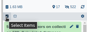
Click on galaxy-selectorSelect Items at the top of the history panel
Check all the datasets in your history you would like to include
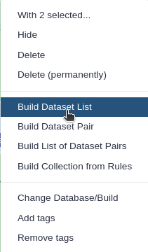
Click n of N selected and choose Advanced Build List
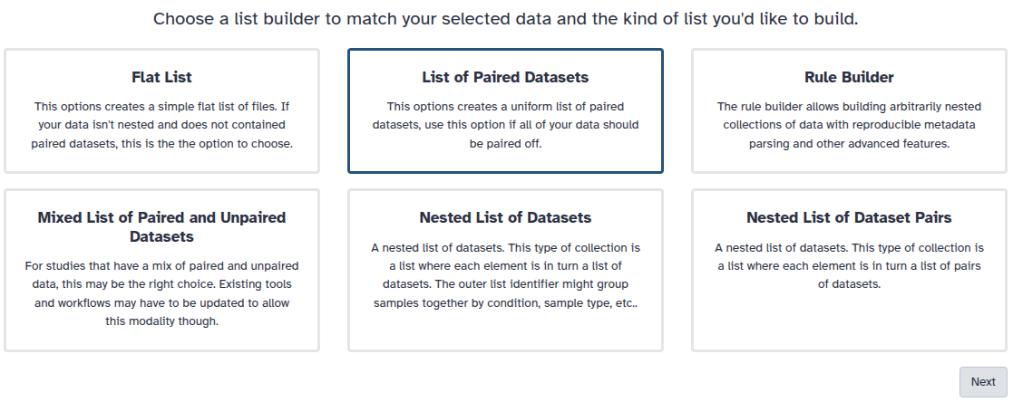
You are in the collection building wizard. Choose List of Paired Datasets and click ‘Next’ button at the right bottom corner.
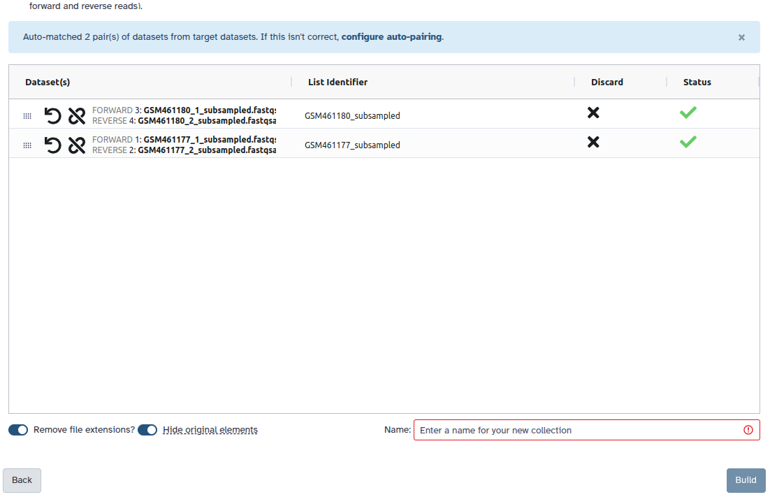
Check and configure auto-pairing. Commonly matepairs have suffix _1 and _2 or _R1 and _R2. Click on ‘Next’ at the bottom.
Edit the List Identifier as required.
Enter a name for your collection
Click Build to build your collection
Click on the checkmark icon at the top of your history again
If you are not familiar with BED format or encode narrowPeak format, see the BED Format
We will visualise regions later in the analysis and obtain the gene information now. We will get information for chromosome 22 genes (names of transcripts and genomic positions) using the UCSC tool.
Hands On: Obtain Annotation for hg38 genes
UCSC Main table browser with the following parameters:
“clade”: Mammal
“genome”: Human
“assembly”: Dec. 2013 (GRCh38/hg38)
“group”: Genes and Gene Prediction
“track”: All GENCODE V37
“table”: Basic
“region”: positionchr22
“output format”: all fields from selected table
“Send output to”: Galaxy
Click get output
Click Send query to Galaxy
This table contains all the information but is not in a BED format. To transform it into BED format we will cut out the required columns and rearrange:
Cut columns from a table with the following parameters:
“Cut columns”: c3,c5,c6,c13,c12,c4
“Delimited by”: Tab
param-file“From”: UCSC Main on Human: wgEncodeGencodeBasicV37 (chr22:1-50,818,468)
Check the contents of your file, is this as you expect it to be?
Question: Expected output
Our goal here was to convert the data to BED format.
Which columns do you expect in your file? (Tip: read about BED format)
Does your file look like a valid BED format?
We expect at least 3 columns, chromosome - start - end, and possibly more optional columns
Troubleshooting: Is your second column the Strand column?
Make sure you used the correct Cuttool (the one that matches the tool name mentioned in the previous step exactly)
There is another tool with (cut) behind the title, we do NOT want to use this tool in this step.
Tip: Always check your output files to make sure they match your expectations!
Renamegalaxy-pencil the dataset as chr22 genes
Click on the galaxy-pencilpencil icon for the dataset to edit its attributes
In the central panel, change the Name field
Click the Save button
Changegalaxy-pencil its datatype to BED
Click on the galaxy-pencilpencil icon for the dataset to edit its attributes
In the central panel, click galaxy-chart-select-dataDatatypes tab on the top
In the galaxy-chart-select-dataAssign Datatype, select bed from “New Type” dropdown
Tip: you can start typing the datatype into the field to filter the dropdown menu
Click the Save button
Click on the galaxy-eye (eye) icon of the file. It should have now column names and they should match the content.
Comment: Gene file
The chr22 genes BED we produced only contains the start, the end, the name, and the strand of each transcript. It does not contain exon information.
To be able to have the exon information, you could use a GTF file which can be downloaded from the gencode website but this file would include the information for the whole genome and would slow the analysis.
Quality Control
The first step is to check the quality of the reads and the presence of the Nextera adapters. When we perform ATAC-Seq, we can get DNA fragments of about 40 bp if two adjacent Tn5 transposases cut the DNA Adey et al. 2010. This can be smaller than the sequencing length so we expect to have Nextera adapters at the end of those reads. We can assess the reads with FastQC.
Hands On: Task description
Run Flatten collection with the following parameters:
“Input collection”: Paired Reads
Rename the flatten collection: Flat Collection
Run FastQC ( Galaxy version 0.74+galaxy1) with the following parameters:
“Raw read data from your current history”: Flat Collection (Flattened paired end read dataset collection)
Inspect the web page output of FastQCtool for the SRR891268_R1 sample. Check what adapters are found at the end of the reads.
Question
How many reads are in the FASTQ?
Which sections have a warning?
There are 285247 reads.
The 3 steps below have warnings:
Per base sequence content
It is well known that the Tn5 has a strong sequence bias at the insertion site. You can read more about it in Green et al. 2012.
Sequence Duplication Levels
The read library quite often has PCR duplicates that are introduced
simply by the PCR itself. We will remove these duplicates later on.
Overrepresented sequences
One sequence is over represented:
you have 306 reads which are exactly the sequence of the Nextera adapter.
They correspond to adapters amplified head-to-head.
306 is really low (only 0.1% of reads).
Comment: FastQC Results
This is what you should expect from the Adapter Content section:
Figure 2: FastQC screenshot on the Adapter Content section
The FastQC web page Adapter Content section shows the presence of Nextera Transposase Sequence in the reads. We will remove the adapters with Cutadapt.
Trimming Reads
To trim the adapters we provide the Nextera adapter sequences to Cutadapt. These adapters are shown in the image below.
Figure 3: Nextera library with the sequence of adapters
The forward and reverse adapters are slightly different. We will also trim low quality bases at the ends of the reads (quality less than 20). We will only keep reads that are at least 20 bases long. We remove short reads (< 20bp) as they are not useful, they will either be thrown out by the mapping or may interfere with our results at the end.
Hands On: Task description
Cutadapt ( Galaxy version 5.1+galaxy0) with the following parameters:
“Single-end or Paired-end reads?”: Paired-end Collection
param-collection“Paired Collection”: Paired Reads
In “Read 1 Adapters”:
In “3’ (End) Adapters”:
param-repeat“Insert 3’ (End) Adapters”
“Source”: Enter custom sequence
“Enter custom 3’ adapter name (Optional if Multiple output is ‘No’)”: Nextera R1
What percentage of reads are still longer than 20bp after the trimming?
~14%
~99%
Hands On: Check Adapter Removal with FastQC
Run Flatten collection with the following parameters:
“Input collection”: Adapter Trimmed Reads
Rename the flatten collection: Flat Trimmed Reads
Run FastQC ( Galaxy version 0.74+galaxy1) with the following parameters:
“Raw read data from your current history”: Flat Trimmed Reads
Click on the galaxy-eye (eye) icon of the report and read the first lines.
Comment: FastQC Results
Now, you should see under Overrepresented sequences that there is no more overrepresented sequences and under Adapter Content that the Nextera adapters are no longer present.
Figure 5: FastQC screenshot on the adapter content section after cutadapt
However, you may have noticed that you have a new section with warning: Sequence Length Distribution. This is expected as you trimmed part of the reads.
Mapping
Mapping Reads to Reference Genome
Next we map the trimmed reads to the human reference genome. Here we will use Bowtie2. We will extend the maximum fragment length (distance between read pairs) from 500 to 1000 because we know some valid read pairs are from this fragment length. We will use the --very-sensitive parameter to have more chance to get the best match even if it takes a bit longer to run. We will run the end-to-end mode because we trimmed the adapters so we expect the whole read to map, no clipping of ends is needed. Regarding the genome to choose. The hg38 version of the human genome contains alternate loci. This means that some region of the genome are present both in the canonical chromosome and on its alternate loci. The reads that map to these regions would map twice. To be able to filter reads falling into repetitive regions but keep reads falling into regions present in alternate loci, we will map on the Canonical version of hg38 (only the chromosome with numbers, chrX, chrY, and chrM).
Comment: Dovetailing
We will allow dovetailing of read pairs with Bowtie2. This is because adapters are removed by Cutadapt only when at least 3 bases match the adapter sequence, so it is possible that after trimming a read can contain 1-2 bases of adapter and go beyond it’s mate start site. For example, if the first mate in the read pair is: GCTATGAAGAATAGGGCGAAGGGGCCTGCGGCGTATTCGATGTTGAAGCT and the second mate is CTTCAACATCGAATACGCCGCAGGCCCCTTCGCCCTATTCTTCATAGCCT, where both contain 2 bases of adapter sequence, they will not be trimmed by Cutadapt and will map this way:
What percentage of read pairs mapped concordantly?
54.8+42.87=97.67%
Comment: On the number of uniquely mapped.
You might be surprised by the number of uniquely mapped compared to the number of multi-mapped reads (reads mapping to more than one location in the genome).
One of the reasons is that we have used the parameter --very-sensitive. Bowtie2 considers a read as multi-mapped even if the second hit has a much lower quality than the first one.
Another reason is that we have reads that map to the mitochondrial genome. The mitochondrial genome has a lot of regions with similar sequence.
Filtering Mapped Reads
Filter Uninformative Reads
We apply some filters to the reads after the mapping. ATAC-Seq datasets can have a lot of reads that map to the mitchondrial genome because it is nucleosome-free and thus very accessible to Tn5 insertion. The mitchondrial genome is uninteresting for ATAC-Seq so we remove these reads. We also remove reads with low mapping quality and reads that are not properly paired.
Hands On: Filtering of uninformative reads
Filter BAM datasets on a variety of attributes ( Galaxy version 2.4.1) with the following parameters:
param-file“BAM dataset(s) to filter”: Select the output of Bowtie2tool“alignments”
In “Condition”:
param-repeat“Insert Condition”
In “Filter”:
param-repeat“Insert Filter”
“Select BAM property to filter on”: mapQuality
“Filter on read mapping quality (phred scale)”: >=30
param-repeat“Insert Filter”
“Select BAM property to filter on”: isProperPair
“Select properly paired reads”: Yes
param-repeat“Insert Filter”
“Select BAM property to filter on”: reference
“Filter on the reference name for the read”: !chrM
“Would you like to set rules?”: No
Click on the input and the output BAM files of the filtering step. Check the size of the files.
Question
Based on the file size, what proportion of alignments was removed (approximately)?
Which parameter should be modified if you are interested in repetitive regions?
The original BAM file is 28.1 MB, the filtered one is 15.2 MB. Approximately half of the alignments were removed.
You should modify the mapQuality criteria and decrease the threshold.
High numbers of mitochondrial reads can be a problem in ATAC-Seq. Some ATAC-Seq samples have been reported to be 80% mitochondrial reads and so wet-lab methods have been developed to deal with this issue Corces et al. 2017 and Litzenburger et al. 2017. It can be a useful QC to assess the number of mitochondrial reads.
However, it does not predict the quality of the rest of the data. It is just that sequencing reads have been wasted.
To get the number of reads that mapped to the mitochondrial genome (chrM) you can run Samtools idxstats ( Galaxy version 2.0.3) on the output of Bowtie2tool“alignments”.
The columns of the output are: chromosome name, chromosome length, number of reads mapping to the chromosome, number of unaligned mate whose mate is mapping to the chromosome.
The first 2 lines of the result would be (after using Sort ( Galaxy version 1.1.1)):
There are 220 000 reads which map to chrM and 165 000 which map to chr22.
Filter Duplicate Reads
Because of the PCR amplification, there might be read duplicates (different reads mapping to exactly the same genomic region) from overamplification of some regions. As the Tn5 insertion is random within an accessible region, we do not expect to see fragments with the same coordinates. We consider such fragments to be PCR duplicates. We will remove them with Picard MarkDuplicates.
Hands On: Remove duplicates
MarkDuplicates ( Galaxy version 2.18.2.2) with the following parameters:
param-file“Select SAM/BAM dataset or dataset collection”: Select the output of Filtertool“BAM”
“If true do not write duplicates to the output file instead of writing them with appropriate flags set”: Yes
Comment: Defaults of MarkDuplicates
By default, the tool will only “Mark” the duplicates. This means that it will change the Flag of the duplicated reads to enable them to be filtered afterwards. We use the parameter “If true do not write duplicates to the output file instead of writing them with appropriate flags set” to directly remove the duplicates.
Click on the galaxy-eye (eye) icon of the MarkDuplicate metrics.
Comment: MarkDuplicates Results
You should get similar output to this from MarkDuplicates:
Once again, if you have a high number of replicates it does not mean that your data are not good, it just means that you sequenced too much compared to the diversity of the library you generated. Consequently, libraries with a high portion of duplicates should not be resequenced as this would not increase the amount of data.
Check Insert Sizes
We will check the insert sizes with Paired-end histogram of insert size frequency. The insert size is the distance between the R1 and R2 read pairs. This tells us the size of the DNA fragment the read pairs came from. The fragment length distribution of a sample gives a very good indication of the quality of the ATAC-Seq.
Hands On: Plot the distribution of fragment sizes.
Paired-end histogram ( Galaxy version 1.0.1) with the following parameters:
param-file“BAM file”: Select the output of MarkDuplicatestool“BAM output”
“Lower bp limit (optional)”: 0
“Upper bp limit (optional)”: 1000
Click on the galaxy-eye (eye) icon of the lower one of the 2 outputs (the png file).
Comment: CollectInsertSizeMetrics Results
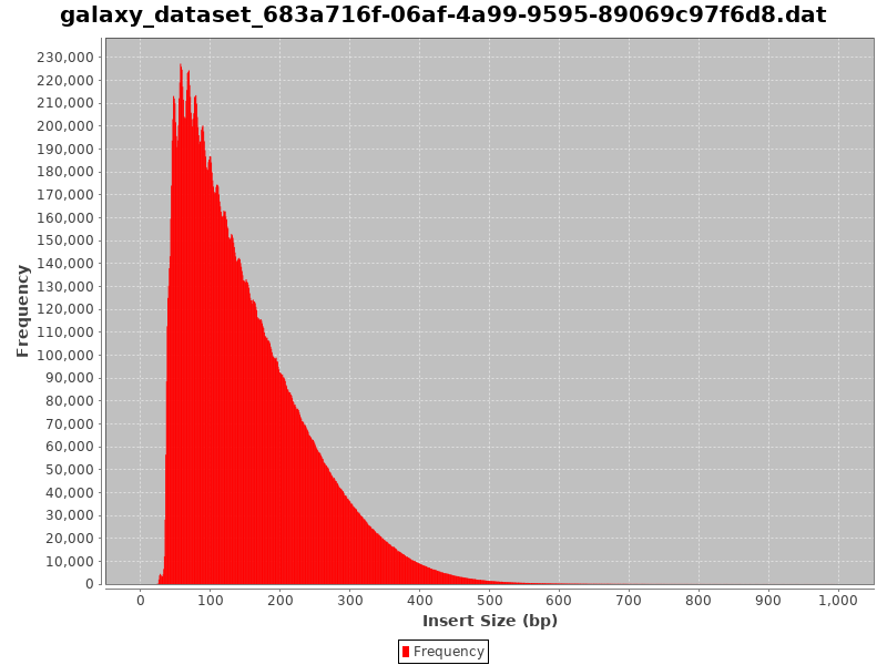
This is what you get from CollectInsertSizeMetrics:
Could you guess what the peaks at approximately 50bp, 200bp, 400bp and 600bp correspond to?
The first peak (50bp) corresponds to where the Tn5 transposase inserted into nucleosome-free regions. The second peak (a bit less than 200bp) corresponds to where Tn5 inserted around a single nucleosome. The third one (around 400bp) is where Tn5 inserted around two adjacent nucleosomes and the fourth one (around 600bp) is where Tn5 inserted around three adjacent nucleosomes.
This fragment size distribution is a good indication if your experiment worked or not.
In absence of chromatin (without nucleosome), this is the profile you would get:
Figure 14: Fragment size distribution of a good ATAC-Seq
Peak calling
Call Peaks
We have now finished the data preprocessing. Next, in order to find regions corresponding to potential open chromatin regions, we want to identify regions where reads have piled up (peaks) greater than the background read coverage. The tools which are currently used are Genrich and MACS2. MACS2 is more widely used. Genrich has a mode dedicated to ATAC-Seq but is still not published and the more reads you have, the less peaks you get (see the issue Genrich#33). That’s why we will not use Genrich in this tutorial.
At this step, two approaches exists:
The first one is to select only paired whose fragment length is below 100bp corresponding to nucleosome-free regions and to use a peak calling like you would do for a ChIP-seq, joining signal between mates. The disadvantages of this approach is that you can only use it if you have paired-end data and you will miss small open regions where only one Tn5 bound.
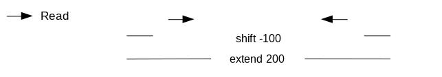
The second one chosen here is to use all reads to be more exhaustive. In this approach, it is very important to re-center the signal of each reads on the 5’ extremity (read start site) as this is where Tn5 cuts. Indeed, you want your peaks around the nucleosomes and not directly on the nucleosome:
This means in order to have the read start site reflecting the centre of where Tn5 bound, the reads on the positive strand should be shifted 4 bp to the right and reads on the negative strands should be shifted 5 bp to the left as in Buenrostro et al. 2013. Genrich can apply these shifts when ATAC-seq mode is selected. In most cases, we do not have 9bp resolution so we don’t take it into account but if you are interested in the footprint, this is important.
If we only assess the coverage of the 5’ extremity of the reads, the data would be too sparse and it would be impossible to call peaks. Thus, we will extend the start sites of the reads by 200bp (100bp in each direction) to assess coverage.
Using MACS2
We convert the BAM file to BED format because when we set the extension size in MACS2, it will only consider one read of the pair while here we would like to use the information from both.
Hands On: Convert the BAM to BED
bedtools BAM to BED converter ( Galaxy version 2.30.0) with the following parameters:
param-file“Convert the following BAM file to BED”: Select the output of MarkDuplicatestool
We call peaks with MACS2. In order to get the coverage centered on the 5’ extended 100bp each side we will use --shift -100 and --extend 200:
MACS2 callpeak ( Galaxy version 2.1.1.20160309.6) with the following parameters:
“Are you pooling Treatment Files?”: No
param-file Select the output of bedtools BAM to BED converter tool
“Do you have a Control File?”: No
“Format of Input Files”: Single-end BED
“Effective genome size”: H. sapiens (2.7e9)
“Build Model”: Do not build the shifting model (--nomodel)
“Set extension size”: 200
“Set shift size”: -100. It needs to be - half the extension size to be centered on the 5’.
“Additional Outputs”:
Check Peaks as tabular file (compatible with MultiQC)
Check Peak summits
Check Scores in bedGraph files
In “Advanced Options”:
“Composite broad regions”: No broad regions
“Use a more sophisticated signal processing approach to find subpeak summits in each enriched peak region”: Yes
“How many duplicate tags at the exact same location are allowed?”: all
Comment: Why keeping all duplicates is important
We previously removed duplicates using MarkDuplicatestool using paired-end information. If two pairs had identical R1 but different R2, we knew it was not a PCR duplicate. Because we converted the BAM to BED we lost the pair information. If we keep the default (removing duplicates) one of the 2 identical R1 would be filtered out as duplicate.
Visualisation of Coverage
Prepare the Datasets
Extract CTCF peaks on chr22 in intergenic regions
As our training dataset is focused on chromosome 22 we will only use the CTCF peaks from chr22. We expect to have ATAC-seq coverage at TSS but only good ATAC-seq have coverage on intergenic CTCF. Indeed, the CTCF protein is able to position nucleosomes and creates a region depleted of nucleosome of around 120bp Fu et al. 2008. This is smaller than the 200bp nucleosome-free region around TSS and also probably not present in all cells. Thus it is more difficult to get enrichment. In order to get the list of intergenic CTCF peaks of chr22, we will first select the peaks on chr22 and then exclude the one which overlap with genes.
Hands On: Select CTCF peaks from chr22 in intergenic regions:
Filter data on any column using simple expressions with the following parameters:
param-file“Filter”: Select the first dataset: ENCFF933NTR.bed.gz
“With following condition”: c1=='chr22'
bedtools Intersect intervals find overlapping intervals in various ways ( Galaxy version 2.30.0) with the following parameters:
param-file“File A to intersect with B”: Select the output of Filter data on any column using simple expressions tool
“Combined or separate output files”: One output file per 'input B' file
param-file“File B to intersect with A”: Select the dataset chr22 genes
“What should be written to the output file?”: Write the original entry in A for each overlap (-wa)
“Required overlap”: Default: 1bp
“Report only those alignments that do not overlap with file(s) B”: Yes
Rename the datasets intergenic CTCF peaks chr22.
Convert bedgraph from MACS2 to bigwig
The bedgraph format is easily readable for human but it can be very large and visualising a specific region is quite slow. We will change it to bigwig format which is a binary format, so we can visualise any region of the genome very quickly.
In this tutorial we focus on chr22, thus we could restrict our bedgraph to chr22 before doing the conversion. This will both speed-up the conversion and decrease the amount of memory needed.
To do so, we will use Filter data on any column using simple expressions with the following parameters:
param-file“Filter”: Select the output of MACS2tool (Bedgraph Treatment).
“With following condition”: c1=='chr22'
This will decrease by half the size of the file.
In the next step, choose the output of Filter instead of the output of MACS2.
Hands On: Convert bedgraphs to bigWig.
Wig/BedGraph-to-bigWig with the following parameters:
param-file“Convert”: Select the output of MACS2tool (Bedgraph Treatment).
“Converter settings to use”: Default
Rename the datasets MACS2 bigwig.
Create heatmap of coverage at TSS with deepTools
You might be interested in checking the coverage on specific regions. For this, you can compute a heatmap. We will use the deepTools plotHeatmap. As an example, we will here make a heatmap centered on the transcription start sites (TSS) and another one centered on intergenic CTCF peaks. First, on the TSS:
Generate computeMatrix
The input of plotHeatmap is a matrix in a hdf5 format. To generate it we use the tool computeMatrix that will evaluate the coverage at each locus we are interested in.
Hands On: Generate the matrix
computeMatrix ( Galaxy version 3.3.2.0.0) with the following parameters:
In “Select regions”:
param-repeat“Insert Select regions”
param-file“Regions to plot”: Select the dataset chr22 genes
“Sample order matters”: No
param-file“Score file”: Select the output of Wig/BedGraph-to-bigWigtool that should be named MACS2 bigwig.
“computeMatrix has two main output options”: reference-point
“The reference point for the plotting”: beginning of region (e.g. TSS)
“Show advanced output settings”: no
“Show advanced options”: yes
“Convert missing values to 0?”: Yes
Plot with plotHeatmap
We will now generate a heatmap. Each line will be a transcript. The coverage will be summarized with a color code from red (no coverage) to blue (maximum coverage). All TSS will be aligned in the middle of the figure and only the 2 kb around the TSS will be displayed. Another plot, on top of the heatmap, will show the mean signal at the TSS. There will be one heatmap per bigwig.
Hands On: Generate the heatmap
plotHeatmap ( Galaxy version 3.3.2.0.1) with the following parameters:
param-file“Matrix file from the computeMatrix tool”: Select the output of computeMatrixtool.
In order to visualise a specific region (e.g. the gene RAC2), we can either use a genome browser like IGV or UCSC browser, or use pyGenomeTracks to make publishable figures. We will use pyGenomeTracks.
Hands On: Task description
pyGenomeTracks ( Galaxy version 3.6) with the following parameters:
“Region of the genome to limit the operation”: chr22:37,193,000-37,252,000
In “Include tracks in your plot”:
param-repeat“Insert Include tracks in your plot”
“Choose style of the track”: Bigwig track
“Plot title”: Coverage from MACS2 (extended +/-100bp)
param-file“Track file(s) bigwig format”: Select the output of Wig/BedGraph-to-bigWigtool called MACS2 bigwig.
“Color of track”: Select the color of your choice
“Minimum value”: 0
“height”: 5
“Show visualization of data range”: Yes
param-repeat“Insert Include tracks in your plot”
“Choose style of the track”: NarrowPeak track
“Plot title”: Peaks from MACS2 (extended +/-100bp)
param-file“Track file(s) encodepeak or bed format”: Select the output of MACS2tool (narrow Peaks).
“Color of track”: Select the color of your choice
“display to use”: box: Draw a box
“Plot labels (name, p-val, q-val)”: No
param-repeat“Insert Include tracks in your plot”
“Choose style of the track”: Gene track / Bed track
“Plot title”: Genes
param-file“Track file(s) bed or gtf format”: chr22 genes
“Color of track”: Select the color of your choice
“height”: 5
“Plot labels”: yes
“Put all labels inside the plotted region”: Yes
“Allow to put labels in the right margin”: Yes
param-repeat“Insert Include tracks in your plot”
“Choose style of the track”: NarrowPeak track
“Plot title”: CTCF peaks
param-file“Track file(s) encodepeak or bed format”: Select the first dataset: ENCFF933NTR.bed.gz
“Color of track”: Select the color of your choice
“display to use”: box: Draw a box
“Plot labels (name, p-val, q-val)”: No
param-repeat“Insert Include tracks in your plot”
“Choose style of the track”: X-axis
Click on the galaxy-eye (eye) icon of the output.
Comment: pyGenomeTracks Results
You should get similar to results to this from pyGenomeTracks:
In the ATAC-Seq sample in this selected region we see four peaks detected by MACS2.
How many TSS are accessible in the sample in the displayed region?
How many CTCF binding loci are accessible?
Can you spot peaks with no TSS and no CTCF peak?
In total, we can see 3 TSS for 6 transcripts for 2 genes. The TSS of RAC2 corresponds to an ATAC-Seq peak whereas there is no significant coverage on both TSS of SSTR3.
Only the first peak on the left overlaps with a CTCF binding site.
Amongst the 4 peaks in this region, the 2 in the middle do not correspond to CTCF peaks or TSS.
As CTCF creates accessible regions, a region containing a peak with no corresponding CTCF peak or TSS could be a putative enhancer. In the pyGenomeTracks plot we see a region like this located in the intron of a gene and another one between genes. However, it is impossible to guess from the position which would be the gene controlled by this region. And of course, more analyses are needed to assess if it is a real enhancer, for example, histone ChIP-seq, 3D structure, transgenic assay, etc.
Conclusion
In this training you have learned the general principles of ATAC-Seq data analysis. ATAC-Seq
is a method to investigate the chromatin accessibility and the genome is treated with
a transposase (enzyme) called Tn5. It marks open chromatin regions by cutting and
inserting adapters for sequencing. The training material gave you an insight into how to quality control the data. You should look for low quality bases, adapter contamination, correct insert size and PCR duplicates (duplication level). We showed you how to remove adapters and PCR duplicates, if FastQC, shows a warning in these areas. We mapped the reads
with Bowtie2, filtered our reads for properly paired, good quality and reads that do not
map to the mitochondrial genome. We found open chromatin regions with MACS2, a tool to find regions of genomic enrichment (peaks). We investigated the read coverage around TSS with the help of computeMatrix and plotHeatmap. Last but not least, we visualised the peaks and other informative tracks, such as CTCF binding regions and hg38 genes, with the help of pyGenomeTracks. At the end, we found open chromatin regions that did not overlap with CTCF sites or TSS, which could be potential putative enhancer regions detected by the ATAC-Seq experiment.
Fu, Y., M. Sinha, C. L. Peterson, and Z. Weng, 2008 The insulator binding protein CTCF positions 20 nucleosomes around its binding sites across the human genome. PLoS genetics 4: e1000138. 10.1371/journal.pgen.1000138
Adey, A., H. G. Morrison, A. (no last name), X. Xun, J. O. Kitzman et al., 2010 Rapid, low-input, low-bias construction of shotgun fragment libraries by high-density in vitro transposition. Genome Biology 11: R119. 10.1186/gb-2010-11-12-r119
Green, B., C. Bouchier, C. Fairhead, N. L. Craig, and B. P. Cormack, 2012 Insertion site preference of Mu, Tn5, and Tn7 transposons. Mobile DNA 3: 3. 10.1186/1759-8753-3-3
Buenrostro, J. D., P. G. Giresi, L. C. Zaba, H. Y. Chang, and W. J. Greenleaf, 2013 Transposition of native chromatin for fast and sensitive epigenomic profiling of open chromatin, DNA-binding proteins and nucleosome position. Nature Methods 10: 1213–1218. 10.1038/nmeth.2688
Corces, M. R., A. E. Trevino, E. G. Hamilton, P. G. Greenside, N. A. Sinnott-Armstrong et al., 2017 An improved ATAC-seq protocol reduces background and enables interrogation of frozen tissues. Nature Methods 14: 959–962. 10.1038/nmeth.4396
Kia, A., C. Gloeckner, T. Osothprarop, N. Gormley, E. Bomati et al., 2017 Improved genome sequencing using an engineered transposase. BMC Biotechnology 17: 10.1186/s12896-016-0326-1
Litzenburger, U. M., J. D. Buenrostro, B. Wu, Y. Shen, N. C. Sheffield et al., 2017 Single-cell epigenomic variability reveals functional cancer heterogeneity. Genome Biology 18: 10.1186/s13059-016-1133-7
Feedback
Did you use this material as an instructor? Feel free to give us feedback on how it went.
Did you use this material as a learner or student? Click the form below to leave feedback.
Hiltemann, Saskia, Rasche, Helena et al., 2023 Galaxy Training: A Powerful Framework for Teaching! PLOS Computational Biology 10.1371/journal.pcbi.1010752
Batut et al., 2018 Community-Driven Data Analysis Training for Biology Cell Systems 10.1016/j.cels.2018.05.012
@misc{epigenetics-atac-seq,
author = "Lucille Delisle and Maria Doyle and Florian Heyl",
	title = "ATAC-Seq data analysis (Galaxy Training Materials)",
	year = "",
	month = "",
	day = "",
	url = "\url{https://training.galaxyproject.org/training-material/topics/epigenetics/tutorials/atac-seq/tutorial.html}",
	note = "[Online; accessed TODAY]"
}
@article{Hiltemann_2023,
	doi = {10.1371/journal.pcbi.1010752},
	url = {https://doi.org/10.1371%2Fjournal.pcbi.1010752},
	year = 2023,
	month = {jan},
	publisher = {Public Library of Science ({PLoS})},
	volume = {19},
	number = {1},
	pages = {e1010752},
	author = {Saskia Hiltemann and Helena Rasche and Simon Gladman and Hans-Rudolf Hotz and Delphine Larivi{\`{e}}re and Daniel Blankenberg and Pratik D. Jagtap and Thomas Wollmann and Anthony Bretaudeau and Nadia Gou{\'{e}} and Timothy J. Griffin and Coline Royaux and Yvan Le Bras and Subina Mehta and Anna Syme and Frederik Coppens and Bert Droesbeke and Nicola Soranzo and Wendi Bacon and Fotis Psomopoulos and Crist{\'{o}}bal Gallardo-Alba and John Davis and Melanie Christine Föll and Matthias Fahrner and Maria A. Doyle and Beatriz Serrano-Solano and Anne Claire Fouilloux and Peter van Heusden and Wolfgang Maier and Dave Clements and Florian Heyl and Björn Grüning and B{\'{e}}r{\'{e}}nice Batut and},
	editor = {Francis Ouellette},
	title = {Galaxy Training: A powerful framework for teaching!},
	journal = {PLoS Comput Biol}
}
Funding
These individuals or organisations provided funding support for the development of this resource
4 stars:
Liked: Clear unambiguous instructions
Disliked: Some tools have many options that were not mentioned in instructions for settings, it would be nice to know for sure that all the options should be left as default, except the ones mentioned in the tutorial. Everything was great up to the resutls of bowtie2. Now I'm not sure if there was some setting that I should have changed, if the settings have been updated/expanded since the tutorial was written? Anyway, in general very happy with this tutorial!
October 2024
4 stars:
Liked: easy to follow
Disliked: show how to use mulitiple replicates
November 2022
4 stars:
Disliked: For the areas where they mention that other analysis options or functions are available please link to other website containing information about those options
March 2022
5 stars:
Liked: The fact that there are explanations for all steps.
Disliked: All were perfect!!!
June 2021
5 stars:
Liked: Everything was explained in detail, easy to follow
May 2021
5 stars:
Liked: The depth of the tutorial, the examples of bad quality data, the explanation why these tools are used and sometimes alternatives, and the overview figure in the conclusion.
April 2021
5 stars:
Liked: Easy to follow
October 2020
4 stars:
Liked: Everything
Disliked: it is good overall
May 2020
5 stars:
Liked: Detailed explanation of each step
Disliked: Comparison of two ATAC-Seq datasets
5 stars:
Liked: Quite easy to follow
Disliked: Bit more interpretation of output
April 2020
5 stars:
Liked: Entire organization, rationale for the steps taken
Disliked: link to smaple out put or all steps like EMBOSS tutorial does
March 2020
5 stars:
Liked: The degree of detail. I loved that even the parameters for the different tools were explained. I don't know if this is comparable to a real experiment analysis, but it surely felt as that. Congrats!
Disliked: The Genrich tool is only available at the GalaxyEurope server. It would be nice that a warning would be given at the beginning of the tutorial, so that the whole analysis could be done there and avoid migrating data between Galaxy servers.
4 stars:
Liked: I have to say the full workflow is very useful for the people who did't know this for a long time, thank you so much. but the tool 'Genrich',I did't find it on the Galaxy...
Disliked: I can't find some tools in Galaxy,
February 2020
5 stars:
Liked: so great!!! its so helpful!!!!!
Disliked: nothing.
3 stars:
Liked: The easiness and the clarity of the examples provided.
Disliked: A print version of the tutorial or pdf to save for offline use.
December 2019
5 stars:
Liked: a good resource for a training session
Disliked: too many steps where you have to 'prepare' data, e.g. sorting the provided bed file
Questions:
 Open image in new tab

Open image in new tab
 Open image in new tab
Open image in new tab
Open image in new tab
Open image in new tab
Open image in new tab
Open image in new tab
Open image in new tab
Open image in new tab
 Open image in new tab
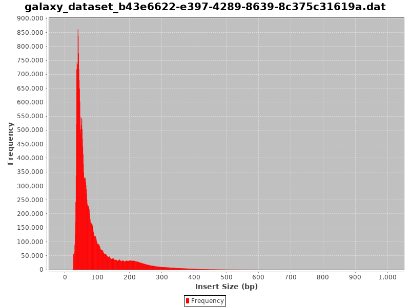 Open image in new tab
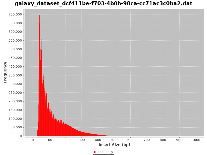 Open image in new tab
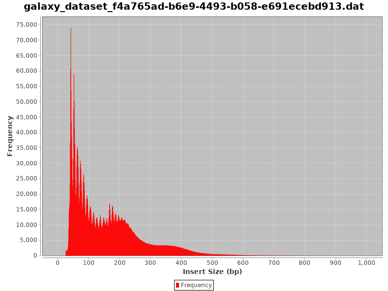 Open image in new tab
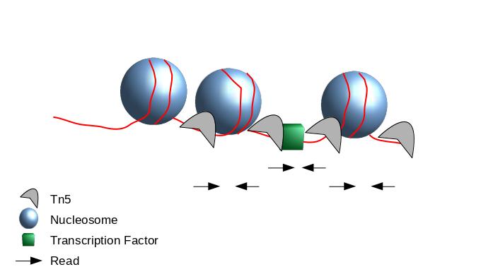 Open image in new tab
Open image in new tab
 Open image in new tab
Open image in new tab
Open image in new tab
Open image in new tab