Image data in medical imaging is often stored and exchanged in the DICOM file format. A DICOM dataset is a file that contains rich metadata (patient, study info) and the actual medical image data stored as pixels (for 2-D images) or voxel (for 3-D images). The image data can be single-channel or multi-channel, and it can also be organized in multiple frames (e.g., spatial tiles of a mosaic, z-slices of a 3-D image, or time steps).
Even though, technically, DICOM datasets can contain heterogeneous frames for different axes (e.g., z-slices and temporal frames), in practice, the frames of a DICOM dataset are usually designated for only one specific purpose and axis (e.g., single z-slices or temporal frames). For such cases, DICOM series are more widely adopted: A list of DICOM datasets can form a DICOM series to store multi-dimensional data (e.g., a list of 3-D images for consecutive time steps, or just the z-slices of a 3-D image, where each slice is a single DICOM dataset).
In this tutorial, we will show how DICOM series and DICOM datasets can be converted to TIFF, which is a general-purpose image file format that is well-supported by a majority of tools in Galaxy. We will use that to showcase segmentation and visualization of anatomical structures in 3-D image data from computed tomography (CT). The Galaxy Image Analysis tools and techniques utilized in this tutorial are domain-agnostic and can also be adapted to other imaging modalities (e.g., 3-D cell imaging).
Rename galaxy-pencil the dataset collection to DICOM series
Click on the galaxy-pencilpencil icon for the dataset to edit its attributes
In the central panel, change the Name field
Click the Save button
Change the datatype of galaxy-pencilDICOM series to Auto-detect
Click on galaxy-selectorSelect Items at the top of the history panel
Check the DICOM series dataset collection
Click 1 of N selected and choose Change data type
In the drop-down field, select Auto-detect
tip: you can start typing the data type into the field to filter the dropdown menu
Click the OK button
Pre-processing
In this DICOM series, each DICOM dataset contains the z-slice of the 3-D image. The metadata of each DICOM dataset in the series contains the z-position of the slice, so the order of the individual DICOM datasets in the collection does not matter (note that for other images, in general, this information might be missing in the metadata, in which case the order of the datasets might be crucial).
Our first step will be to convert the DICOM series into a single TIFF image, that represents the whole 3-D dataset.
Hands On: Convert DICOM series to TIFF image
Convert DICOM to TIFF ( Galaxy version 0.27.0+galaxy0) with the following parameters to convert the DICOM series (list of DICOM datasets) into a list of TIFF images:
param-files“DICOM dataset”: DICOM series collection
Concatenate images or channels ( Galaxy version 0.5) with the following parameters to concatenate the stack of TIFF images along the z-axis into a single 3-D image:
param-files“Images to concatenate”: Output of Convert DICOM to TIFF ( Galaxy version 0.27.0+galaxy0)
“Concatenation axis”: Z-axis (concatenate images as slices of a 3-D image or image sequence)
“Scaling of values”: Preserve range of values
“Sort images before concatenating”: Sort images by their position along the Z-axis
Comment: Why do we convert DICOM to TIFF?
Although DICOM is the standard file format in medical imaging, in research, it is convenient to use to TIFF for image analysis for several reasons:
Advantages of TIFF for image analysis:
Tool compatibility: Most image analysis and visualization tools in Galaxy and other scientific computing platforms are optimized for standard, general-purpose image formats like TIFF. In addition, TIFF is also well-supported by programming languages (e.g., Python, MATLAB), which can be handy for advanced analyses.
Simpler structure: TIFF has more straightforward data organization for computational processing. A single multi-dimensional TIFF file is easier to handle than hundreds or thousands of separate DICOM datasets.
Metadata handling: The extensive clinical metadata of DICOM (e.g., patient info, acquisition protocols) can be challenging to parse and process for general-purpose image analysis tools.
Important considerations:
Metadata preservation is critical: During conversion, spatial calibration data (voxel spacing, slice positions, orientation) must be preserved. Without these informations, it is not possible to translate spatial image analysis readouts (e.g., object sizes) into physical units (e.g., mm, cm), rendering quantitative analysis meaningless.
DICOM advantages: DICOM remains essential for clinical workflows, PACS integration, and regulatory compliance. For pure clinical use, stay in DICOM format.
Some of the tools that we will be using in our analysis require that the voxel size of the image is isotropic. To ensure that this is the case, we will re-sample the image data to an isotropic voxel size:
Hands On: Re-sample image data for isotropic pixel/voxel sizes
Scale image ( Galaxy version 0.25.2+galaxy0) with the following parameters to re-sample the image data to an isotropic voxel size:
param-file“Input image”: Output of Concatenate images or channels ( Galaxy version 0.5)
“How to scale?”: Scale to spatially isotropic pixels/voxels
“Method”: Down-sample (might lose information)
If the image data already would have been isotropic, this tool would yield the original data.
CT image data, such as the dataset used in this tutorial, typically has intensity values that correspond to the Hounsfield scale:
The Hounsfield scale, named after Sir Godfrey Hounsfield, is a quantitative scale for describing radiodensity. It is frequently used in CT scans, where its value is also termed CT number.
Using Hounsfield Units (HU) is advantageous, because it allows to directly identify specific materials or tissues solely based on the image intensities. Typical Hounsfield unit (HU) values are −1000 HU for air, approximately −950 to −650 HU for normally aerated lung tissue, −190 to −30 HU for subcutaneous fat, 0 HU for water, +30 to +60 HU for muscle tissue, and >+150 HU for bone tissue (often >+1000 HU for cortical bone; e.g., Chougule et al. 2017, Lim Fat et al. 2011). In research, often larger ranges are used to account for pathological cases or contrast enhancement (e.g., –29 to +150 HU for muscle tissue).
The image data may also contain values outside of the range of –1000 to 3071 HU that correspond to, for example, parts of the CT imaging setup, or imaging artifacts. To effectively “erase” those parts from the image data, we will clip the image intensities to the meaningful range of –1000 to 3071 HU as a final step of pre-processing:
Hands On: Clipping the image intensities
Clip image intensities ( Galaxy version 0.7.3+galaxy0) with the following parameters:
param-file“Input image”: Output of Scale image ( Galaxy version 0.25.2+galaxy0)
“Lower bound”: -1000
“Upper bound”: 3071
Exploring the Image Data
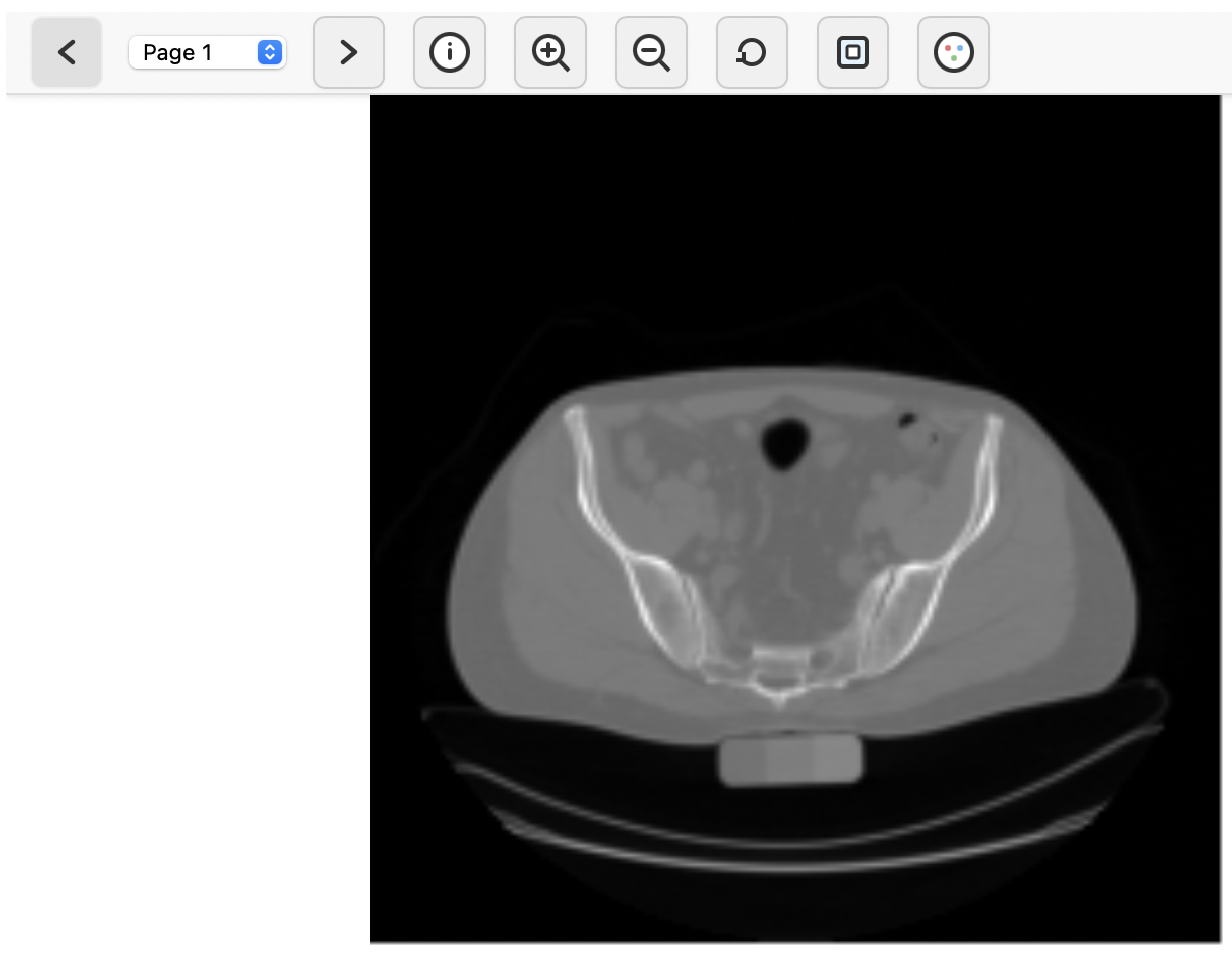
Galaxy’s built-in TIFF viewer can be used to roughly explore the image data. To do so, click on the galaxy-eye (eye) icon next to the output of the Clip image intensities ( Galaxy version 0.7.3+galaxy0) tool. This will bring up a basic user interface that shows a z-slice of the 3-D image, along with the option to navigate to a different slice along the z-axis (slices are presented as “pages”). The viewer shows the x-axis as left-to-right and the y-axis as top-to-bottom.
The buttons in the toolbar can be used to zoom and pan the view, or this can be accomplished by using the scroll wheel or dragging the image with a pressed mouse button. Even though this viewer is very simple, we can make two important observations that provide some rough orientation within the image data that we are dealing with:
The y-axis is the anteroposterior axis (or anterior-posterior, from the front to the back of the torso).
The z-axis is the craniocaudal axis (or cranial-caudal, from the bottom to the top of the torso).
We will now use this information to get a visually more informative representation of the image data by creating a 3-D volume rendering (geometrical projection of the 3-D image data onto the 2-D screen plane).
Inspecting 3-D data as a 2-D projection is intrinsically challenging because it requires transformations of the data that inherently reduce the information along the way—but we as humans, who are also subject to this limitation due to our two-dimensional vision, we have learned to deal with it naturally by taking looks from different angles. The tool that we are going to use for visualization mimics this intuition by generating videos instead of plain images, that use different angles for the projection:
Hands On: Visual inspection via pre-rendered video
Render 3-D image data ( Galaxy version 0.2.0+galaxy2) with the following parameters:
param-file“Input image (3-D)”: Output of Clip image intensities ( Galaxy version 0.7.3+galaxy0)
“Unit of the intensity values”: Hounsfield
“Rendering mode”: Maximum Intensity Projection (MIP)
“Color map”: rainbow
“Camera parameters”:
“Distance”: 350
“Video parameters”:
“Frames”: 400
Comment: How do we establish proper orientation of the image data in 3-D?
The parameter for the “Coordinate system” is set to Point Z to the top by default. This is the setting that we must use here, since we have identified the z-axis as the craniocaudal axis. For other image data it might be necessary to instead Point Y to the top.
Click on the galaxy-eye (eye) icon next to the output of the Render 3-D image data ( Galaxy version 0.2.0+galaxy2) tool to inspect the obtained visualization:
The Maximum Intensity Projection (MIP) is useful to get an idea of the spatial distribution of the image intensities within the image. At each time step of the video, the MIP is computed by casting a ray from each image pixel through the 3-D volume of image intensities, and taking the maximum intensity value along the line by sampling the image intensities at fixed steps (the rendering technique is thus called ray marching).
Skeletal Segmentation
The imaged section of the torso in our dataset contains parts of prominent skeletal structures such as the pelvis, the spine, and the thorax. Segmentation of these structures is easy due to the distinct ranges of the Hounsfield scale:
Hands On: Skeletal segmentation in a CT image
Threshold image ( Galaxy version 0.25.2+galaxy0) with the following parameters:
param-file“Input image”: Output of Clip image intensities ( Galaxy version 0.7.3+galaxy0)
“Thresholding method”: Manual
“Threshold value”: 120
Question
Why do we use a threshold value of just 120, if the typical range of HU values for bone tissue starts at about 150 HU?
Some bones in the imaged data are quite thin (e.g., the ends of the ribs). This leads to partial volume effects: voxels at the edges of thin structures contain a mixture of bone and surrounding soft tissue (e.g., cartilage), resulting in intermediate intensity values lower than pure bone. When we re-sampled the image data to an isotropic voxel size, we chose to down-sample the image data. A consequence of this is that voxel intensity values are locally averaged, which can lead to reduced intensity values of thin structures.
Lets inspect the segmentation result using a 3-D overlay of the input image and the segmentation mask:
Hands On: Visualization of 3-D segmentation results
Render 3-D image data ( Galaxy version 0.2.0+galaxy2) with the following parameters:
param-file“Input image (3-D)”: Output of Clip image intensities ( Galaxy version 0.7.3+galaxy0)
“Unit of the intensity values”: Hounsfield
“Rendering mode”: Direct Volume Rendering (DVR)
“Color map”: BrBG
“Ramp function”: Enabled
“Ramp start”:
“Type of the intensity value”: Absolute intensity value
“Intensity value”: 100
“Ramp end”:
“Type of the intensity value”: Absolute intensity value
“Intensity value”: 150
“Camera parameters”:
“Distance”: 350
“Render mask overlay”: Render mask overlay
“Mask overlay (3-D)”: Output of Threshold image ( Galaxy version 0.25.2+galaxy0)
“Video parameters”:
“Frames”: 400
The Direct Volume Rendering (DVR) is rendering technique similar to MIP, but instead of taking the maximum intensity for each image pixel it simulates the absorption of light and thus produces realistically looking surface renderings. Click on the galaxy-eye (eye) icon next to the output of the Render 3-D image data ( Galaxy version 0.2.0+galaxy2) tool to inspect the obtained visualization:
It can be seen from the visualization that objects corresponding to parts of the imaging setup (behind the spine) also fall into the selected HU range, and is thus falsely included in the segmentation skeletal segmentation result (leakage). To improve the segmentation result, we will thus remove all objects from the segmentation that are behind the spine and pelvis. To identify the spine and pelvis in the segmentation result, we exploit that they correspond to the largest connected component in our segmentation.
The first step is to determine the sizes of the connected components:
Hands On: Feature extraction for the connected components of the segmentation result
Convert binary image to label map ( Galaxy version 0.7.3+galaxy0) with the following parameters to assign a unique label to each connected component of the segmentation result:
“Mode”: Connected component analysis
param-file“Binary image”: Output of Threshold image ( Galaxy version 0.25.2+galaxy0)
Extract image features ( Galaxy version 0.25.2+galaxy1) with the following parameters to measure the size and location of each connected component:
param-file“Label map”: Output of Convert binary image to label map ( Galaxy version 0.7.3+galaxy0)
“Available features”:
Label from the label map
Area
Centroid
Next, we inspect the tabular output yielded by the Extract image features ( Galaxy version 0.25.2+galaxy1) tool:
label
area
centroid_x
centroid_y
centroid_z
1
61710.0
88.83420839410144
103.37395883973424
36.61537838275806
2
10465.0
97.36292403248925
139.6089823220258
52.41691352126135
3
1.0
87.0
137.0
0.0
4
2.0
44.0
159.0
0.5
5
7.0
132.0
159.0
3.0
6
6.0
48.5
160.0
1.0
…
…
…
…
…
In this table, each row corresponds to a connected component in the segmentation result (identified by its unique label). The centroid of the connected components tells us where the components are located (the y-axis is the anteroposterior axis and points from the front to the back of the torso). By inspecting this table, we can easily conclude that the centroid of the largest connected component is located at a y-coordinate of 103.37 (in voxels).
Since this coordinate corresponds to the centroid of the spine and pelvis, removing all objects with a y-coordinate of more than 103.37 voxels is likely to also remove some ribs—which we do not want to happen. Hence, we will add a tolerance margin for objects: Instead of strictly removing all objects that are behind the centroid of the spine and pelvis, we will only remove those that are 1.5 cm or further behind.
The size of the margin needs to be given in voxels. To determine that, we inspect the standard output of the Scale image ( Galaxy version 0.25.2+galaxy0) tool, that contains many details:
Hands On: Inspect the standard output of the "Scale image" tool
Expand the history item for the output of the Scale image ( Galaxy version 0.25.2+galaxy0) tool.
Click on the details icon.
Scroll down to the Job Information section to view the “Tool Standard Output” log:
Code Out: Standard output of the "Scale image" tool
What we are interested in here is the line for the Output resolution. The first tuple (0.4000000241509449, 0.4000000241509449) corresponds to the number of voxels per millimeter along the x- and y-axes. From this, we can deduce, using basic algebra, that one voxel corresponds to 2.5 mm along the y-axis (in fact, we can also read off the value for the z_spacing, which is identical due to the isotropic re-sampling). Thus, a margin of 1.5 cm corresponds to 6 voxels.
With this information, we can now write a rules file for removing the leakage from the segmentation result:
Hands On: Write a rules file to remove spurious objects from the segmentation
Create a new file via the galaxy-uploadUpload Data tool in Galaxy, use the name rules_skeletal, paste the following content, and set the format to tabular:
feature   	min	max
centroid_y	0	109.37
Click galaxy-uploadUpload Data at the top of the tool panel
Select galaxy-wf-editPaste/Fetch Data at the bottom
Paste the file contents into the text field
Change the dataset name from “New File” to rules_skeletal
Change Type from “Auto-detect” to tabular* Press Start and Close the window
The upper bound of 109.37 for the y-coordinate of the centroids of the objects that we will retain in the segmentation is obtained by adding the margin of 6 voxels to the previously determined y-coordinate of the centroid of the spine and pelvis.
Now we are all set to remove the leakage from the segmentation result:
Hands On: Remove spurious objects from the segmentation
Filter label map by rules ( Galaxy version 0.7.3+galaxy1) with the following parameters:
param-file“Label map”: Output of Convert binary image to label map ( Galaxy version 0.7.3+galaxy0)
param-file“Features”: Output of Extract image features ( Galaxy version 0.25.2+galaxy1)
param-file“Rules”: rules_skeletal
Render 3-D image data ( Galaxy version 0.2.0+galaxy2) with the following parameters:
param-file“Input image (3-D)”: Output of Clip image intensities ( Galaxy version 0.7.3+galaxy0)
“Unit of the intensity values”: Hounsfield
“Rendering mode”: Direct Volume Rendering (DVR)
“Color map”: BrBG
“Ramp function”: Enabled
“Ramp start”:
“Type of the intensity value”: Absolute intensity value
“Intensity value”: 100
“Ramp end”:
“Type of the intensity value”: Absolute intensity value
“Intensity value”: 150
“Camera parameters”:
“Distance”: 350
“Render mask overlay”: Render mask overlay
“Mask overlay (3-D)”: Output of Filter label map by rules ( Galaxy version 0.7.3+galaxy1)
“Video parameters”:
“Frames”: 400
Click on the galaxy-eye (eye) icon next to the output of the Render 3-D image data ( Galaxy version 0.2.0+galaxy2) tool to visually inspect the improved segmentation result:
Question: Further improvements of the segmentation result
The visualization above shows that there are still small, spurious objects included in the segmentation. How to remove these?
Add another rule to the rules_skeletal file that you have created, then re-run the Filter label map by rules ( Galaxy version 0.7.3+galaxy1) tool. That rule should be for the area feature and impose a reasonable min value for the minimum size of retained connected components. The value for max could be 100000, for example.
Vessel Segmentation
As another example of the segmentation of anatomical structures, we will now perform a segmentation of the aortic bifurcation, a key vascular landmark where the abdominal aorta divides into the left and right common iliac arteries. Vessel segmentation is very different from skeletal segmentation, because vessels do not exhibit a specific HU intensity value and generally have a very low contrast compared to the surrounding tissue. Moreover, they often are very thin, elongated structures, with and without branches, which poses additional challenges compared to segmentation of large connected image regions.
In CT imaging, vessels usually appear as thin lines of subtly higher intensity than the surrounding tissue (just like the ridges of mountains on a relief map). Image filters that enhance such structures are thus called ridge filters. The most prominent ridge filter for vessel enhancement in 3-D images is the Frangi filter (Frangi et al. 1998).
Comment: Contrast-enhanced vs. non-contrast vessel imaging
Vessel segmentation feasibility is highly dependent on the imaging protocol:
Non-contrast CT:
Blood vessels: ~30–50 HU (similar to muscle: 40–60 HU)
Can also be much less due to partial volume effects
Minimal contrast with surrounding tissue
Less suited for detailed vascular examination (e.g., segmentation of whole vessel trees)
Frangi filter unreliable for very thin vessels (e.g., coronary vessels)
Contrast-enhanced CT (CTA):
Contrast-filled vessels: 250–400 HU (with iodinated contrast agent)
Excellent contrast against surrounding tissue (40–60 HU)
Frangi filter performs reliably for vessel detection
Clinical standard for vascular imaging and segmentation
The image data used in this tutorial is non-contrast CT.
Our workflow for the segmentation of the aortic bifurcation is as follows:
First, we will apply a Frangi filter to perform image enhancement for vessels and other vessel-like structures. The responses of Frangi filters range between 0 and 1, which directly indicates the “vesselness” of an image point.
Second, we will perform hysteresis thresholding to segment connected parts of the vascular tree with a particularly high filter response (i.e. a particularly high vesselness).
Third, we will apply feature extraction and label map filtering to select the largest connected component of the segmented vascular tree (like we did for skeletal segmentation).
The individual workflow steps are as follows:
Hands On: Vessel segmentation and feature extraction
Apply ridge filter ( Galaxy version 0.22.0+galaxy2) with the following parameters:
param-file“Input image”: Output of Clip image intensities ( Galaxy version 0.7.3+galaxy0)
“Filter”: Frangi vesselness filter
“Mode of operation”: Enhance bright ridges (high image intensities)
“Minimum sigma”: 0.5
“Maximum sigma”: 1.5
“Number of sigma steps for multi-scale analysis”: 3
“Alpha”: 0.5
“Beta”: 0.5
“Gamma”: 5.0
Threshold image ( Galaxy version 0.25.2+galaxy0) with the following parameters:
param-file“Input image”: Output of Apply ridge filter ( Galaxy version 0.22.0+galaxy2)
“Thresholding method”: Manual
“Threshold value”: 0.25
“Second threshold value for hysteresis thresholding”: 0.3
Convert binary image to label map ( Galaxy version 0.7.3+galaxy0) with the following parameters:
“Mode”: Connected component analysis
param-file“Binary image”: Output of Threshold image ( Galaxy version 0.25.2+galaxy0)
Extract image features ( Galaxy version 0.25.2+galaxy1) with the following parameters:
param-file“Label map”: Output of Convert binary image to label map ( Galaxy version 0.7.3+galaxy0)
“Available features”:
Label from the label map
Area
Sort ( Galaxy version 9.5+galaxy2) with the following parameters:
param-file“Sort Query”: Output of Extract image features ( Galaxy version 0.25.2+galaxy1)
“Number of header lines”: 1
“Column selections”: 1: Column selections
“on column”: Column 2
“in”: Descending order
“Flavor”: Fast numeric sort (-n)
We inspect the tabular output yielded by the Sort ( Galaxy version 9.5+galaxy2) tool:
label
area
26
11167.0
132
8739.0
176
2910.0
175
2821.0
42
2157.0
…
…
From this table, we can deduce that the largest connected component is the one with label 26. We now create the corresponding rules file for removing all other components from the segmentation:
Hands On: Segmentation and visualization of the aortic bifurcation
Create a new file via the galaxy-uploadUpload Data tool in Galaxy, use the name rules_aorticbif, paste the following content, and set the format to tabular:
feature	min	max
label  	26	26
Click galaxy-uploadUpload Data at the top of the tool panel
Select galaxy-wf-editPaste/Fetch Data at the bottom
Paste the file contents into the text field
Change the dataset name from “New File” to rules_aorticbif
Change Type from “Auto-detect” to tabular* Press Start and Close the window
Filter label map by rules ( Galaxy version 0.7.3+galaxy1) with the following parameters:
param-file“Label map”: Output of Convert binary image to label map ( Galaxy version 0.7.3+galaxy0)
param-file“Features”: Output of Extract image features ( Galaxy version 0.25.2+galaxy1)
param-file“Rules”: rules_aorticbif
Create a new file via the galaxy-uploadUpload Data tool in Galaxy, use the name colormap_white, paste the following content, and set the format to tabular:
color	intensity	type
#ffffff00	0	relative
#ffffffff	1 	relative
Click galaxy-uploadUpload Data at the top of the tool panel
Select galaxy-wf-editPaste/Fetch Data at the bottom
Paste the file contents into the text field
Change the dataset name from “New File” to colormap_white
Change Type from “Auto-detect” to tabular* Press Start and Close the window
Render 3-D image data ( Galaxy version 0.2.0+galaxy2) with the following parameters:
param-file“Input image (3-D)”: Output of Filter label map by rules ( Galaxy version 0.7.3+galaxy1)
“Unit of the intensity values”: No unit
“Rendering mode”: Direct Volume Rendering (DVR)
“Color map”: Custom
param-file“Custom color map”: colormap_white
“Add a color bar”: No
“Camera parameters”:
“Distance”: 250
“Render mask overlay”: No overlay
“Video parameters”:
“Frames”: 400
The obtained visualization shows the segmentation of the aortic bifurcation:
Vessel segmentation is generally challenging and still an active field of research. Segmentation of whole vascular trees may require more sophisticated methods (e.g., Gülsün and Tek 2008, Biesdorf et al. 2015).
Fully automated workflow
This tutorial contained several interactive steps that required inspection of data from previous steps. Note that this steps can also be automated, as we show in the supplemental workflow:
Click on galaxy-workflows-activityWorkflows in the Galaxy activity bar (on the left side of the screen, or in the top menu bar of older Galaxy instances). You will see a list of all your workflows
Click on galaxy-uploadImport at the top-right of the screen
Paste the following URL into the box labelled “Archived Workflow URL”: https://training.galaxyproject.org/training-material/topics/imaging/tutorials/dicom-anatomical-3d/workflows/dicom-anatomical-3d.ga
Click the Import workflow button
Below is a short video demonstrating how to import a workflow from GitHub using this procedure:
Video: Importing a workflow from URL
You've Finished the Tutorial
Please also consider filling out the Feedback Form as well!
Key points
DICOM images are best converted to TIFF that is well supported by a majority of image analysis tools in Galaxy.
Computed tomography images usually permit direct identification of materials and tissues based on the intensity values.
Ridge filters help enhancing and segmenting thin, elongated structures, such as vessels.
Frequently Asked Questions
Have questions about this tutorial? Have a look at the available FAQ pages and support channels
Further information, including links to documentation and original publications, regarding the tools, analysis techniques and the interpretation of results described in this tutorial can be found here.
References
Frangi, A. F., W. J. Niessen, K. L. Vincken, and M. A. Viergever, 1998 Multiscale vessel enhancement filtering, pp. 130–137 inMedical Image Computing and Computer-Assisted Intervention — MICCAI’98, Springer Berlin Heidelberg. 10.1007/bfb0056195 ISBN: 9783540495635
Gülsün, M. A., and H. Tek, 2008 Robust Vessel Tree Modeling, pp. 602–611 inMedical Image Computing and Computer-Assisted Intervention – MICCAI 2008, Springer Berlin Heidelberg. 10.1007/978-3-540-85988-8_72 ISBN: 9783540859888
Lim Fat, D., J. Kennedy, R. Galvin, F. O’Brien, F. Mc Grath et al., 2011 The Hounsfield value for cortical bone geometry in the proximal humerus—an in vitro study. Skeletal Radiology 41: 557–568. 10.1007/s00256-011-1255-7
Biesdorf, A., S. Wörz, H. von Tengg-Kobligk, K. Rohr, and C. Schnörr, 2015 3D segmentation of vessels by incremental implicit polynomial fitting and convex optimization, pp. 1540–1543 in2015 IEEE 12th International Symposium on Biomedical Imaging (ISBI), IEEE. 10.1109/isbi.2015.7164171
Did you use this material as an instructor? Feel free to give us feedback on how it went.
Did you use this material as a learner or student? Click the form below to leave feedback.
Hiltemann, Saskia, Rasche, Helena et al., 2023 Galaxy Training: A Powerful Framework for Teaching! PLOS Computational Biology 10.1371/journal.pcbi.1010752
Batut et al., 2018 Community-Driven Data Analysis Training for Biology Cell Systems 10.1016/j.cels.2018.05.012
@misc{imaging-dicom-anatomical-3d,
author = "Leonid Kostrykin",
	title = "Segmentation of Anatomical Structures in Medical 3-D Images (Galaxy Training Materials)",
	year = "",
	month = "",
	day = "",
	url = "\url{https://training.galaxyproject.org/training-material/topics/imaging/tutorials/dicom-anatomical-3d/tutorial.html}",
	note = "[Online; accessed TODAY]"
}
@article{Hiltemann_2023,
	doi = {10.1371/journal.pcbi.1010752},
	url = {https://doi.org/10.1371%2Fjournal.pcbi.1010752},
	year = 2023,
	month = {jan},
	publisher = {Public Library of Science ({PLoS})},
	volume = {19},
	number = {1},
	pages = {e1010752},
	author = {Saskia Hiltemann and Helena Rasche and Simon Gladman and Hans-Rudolf Hotz and Delphine Larivi{\`{e}}re and Daniel Blankenberg and Pratik D. Jagtap and Thomas Wollmann and Anthony Bretaudeau and Nadia Gou{\'{e}} and Timothy J. Griffin and Coline Royaux and Yvan Le Bras and Subina Mehta and Anna Syme and Frederik Coppens and Bert Droesbeke and Nicola Soranzo and Wendi Bacon and Fotis Psomopoulos and Crist{\'{o}}bal Gallardo-Alba and John Davis and Melanie Christine Föll and Matthias Fahrner and Maria A. Doyle and Beatriz Serrano-Solano and Anne Claire Fouilloux and Peter van Heusden and Wolfgang Maier and Dave Clements and Florian Heyl and Björn Grüning and B{\'{e}}r{\'{e}}nice Batut and},
	editor = {Francis Ouellette},
	title = {Galaxy Training: A powerful framework for teaching!},
	journal = {PLoS Comput Biol}
}
Funding
These individuals or organisations provided funding support for the development of this resource
Questions:

 Open image in new tab
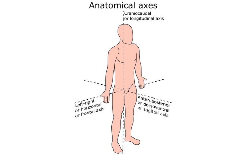 Open image in new tab
