Phylogenetics - Back to Basics - Building Trees

Contributors

Authors: Michael Charleston

Why build trees?

The main reason we end up building a tree is that searching tree space for an optimal one takes too long when the number of taxa gets large.
.reduce70[ | n | # trees | yes, but how much is that really? | — |—|:–| | 3 | 3 | enumerable by hand | | 4 | 15 | enumerable by hand | | 5 | 105 | enumerable by hand on a rainy day | | 6 | 945 | enumerable by computer | | 7 | 10395 | still searchable very quickly on computer | | 8 | 135135 | a bit more than the number of hairs on your head | | 9 | 2027025 | population of Sydney living west of Parramatta | | 10 | 34459425 | \(\approx\) upper limit for exhaustive searching; about the number of possible combinations of numbers in the National Lottery | | 20 | \(8.2\times 10^{21}\) | \( \approx \) upper limit for branch-and-bound searching | | 48 | \(3.21 \times 10^{70}\) | \(\approx\) number of particles in the universe | | 136 | \(2.11 \times 10^{267}\) | number of trees to choose from in the ``Out of Africa’’ data¹ | ]

.footnote[ ¹ Vigilant et al., 1991 ]

Tree space is worse than “space” space

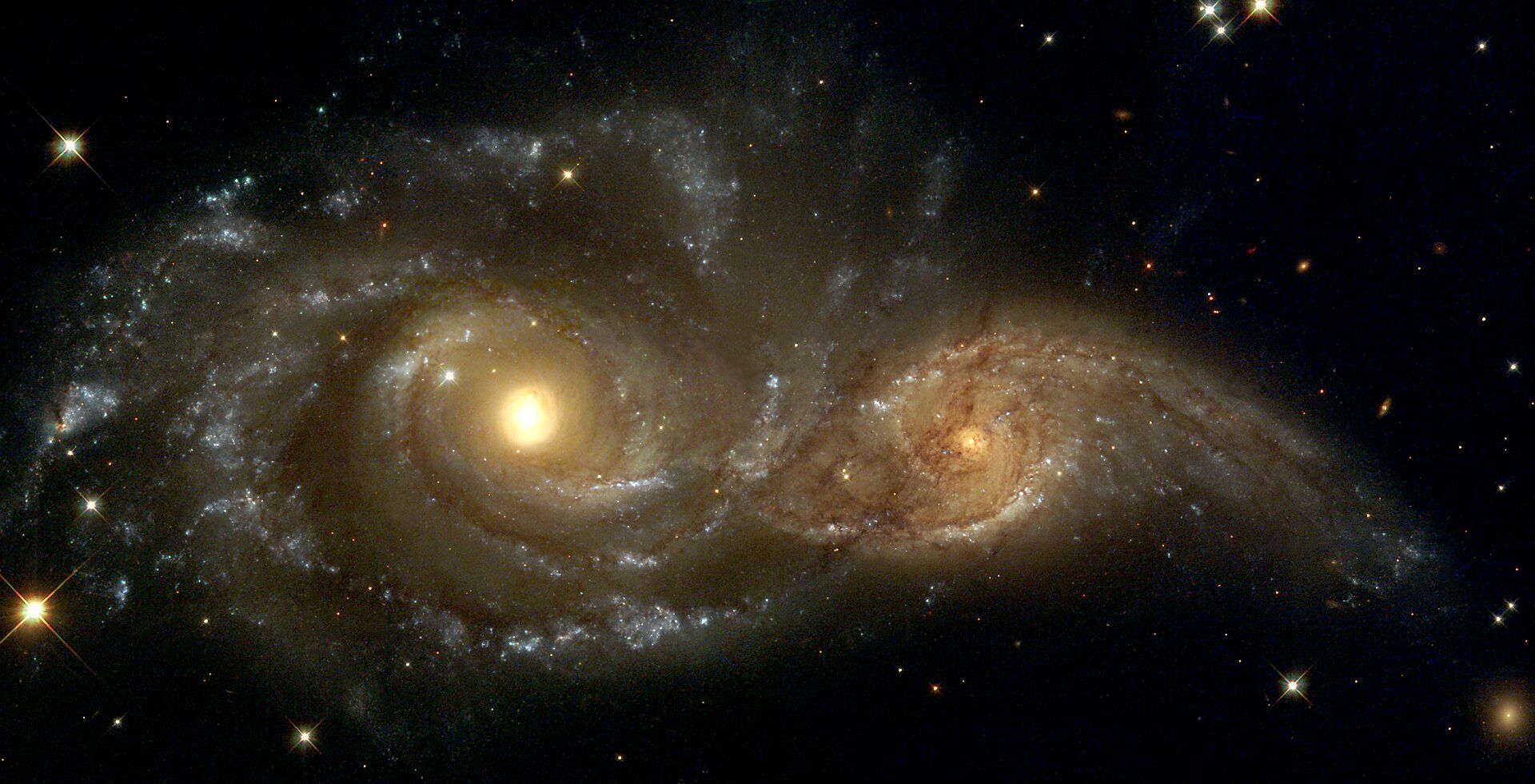
NGC 2207 and IC 2163 galaxies colliding.
.footnote[Source: https://commons.wikimedia.org/wiki/Commons:Featured_pictures/Astronomy] —

Why should building work then?

Some parts of a phylogeny can be confidently accepted: when there are two species much more similar to each other than they are to any other species, we can confidently say that they are likely to be each other’s closest relatives, in the set of species of interest.

If molecular sequences evolve at a nice steady rate - the “molecular clock” hypothesis - and if there’s neither too little nor too much change, this can be good enough.

Distances from trees

Before we talk about building a tree from distances, we need to think about how distances are reflected by trees.

The most natural way to infer distances from trees is by adding the lengths of branches between each pair of nodes.

Such distances are called patristic distances (I don’t know why). —

Patristic Distances

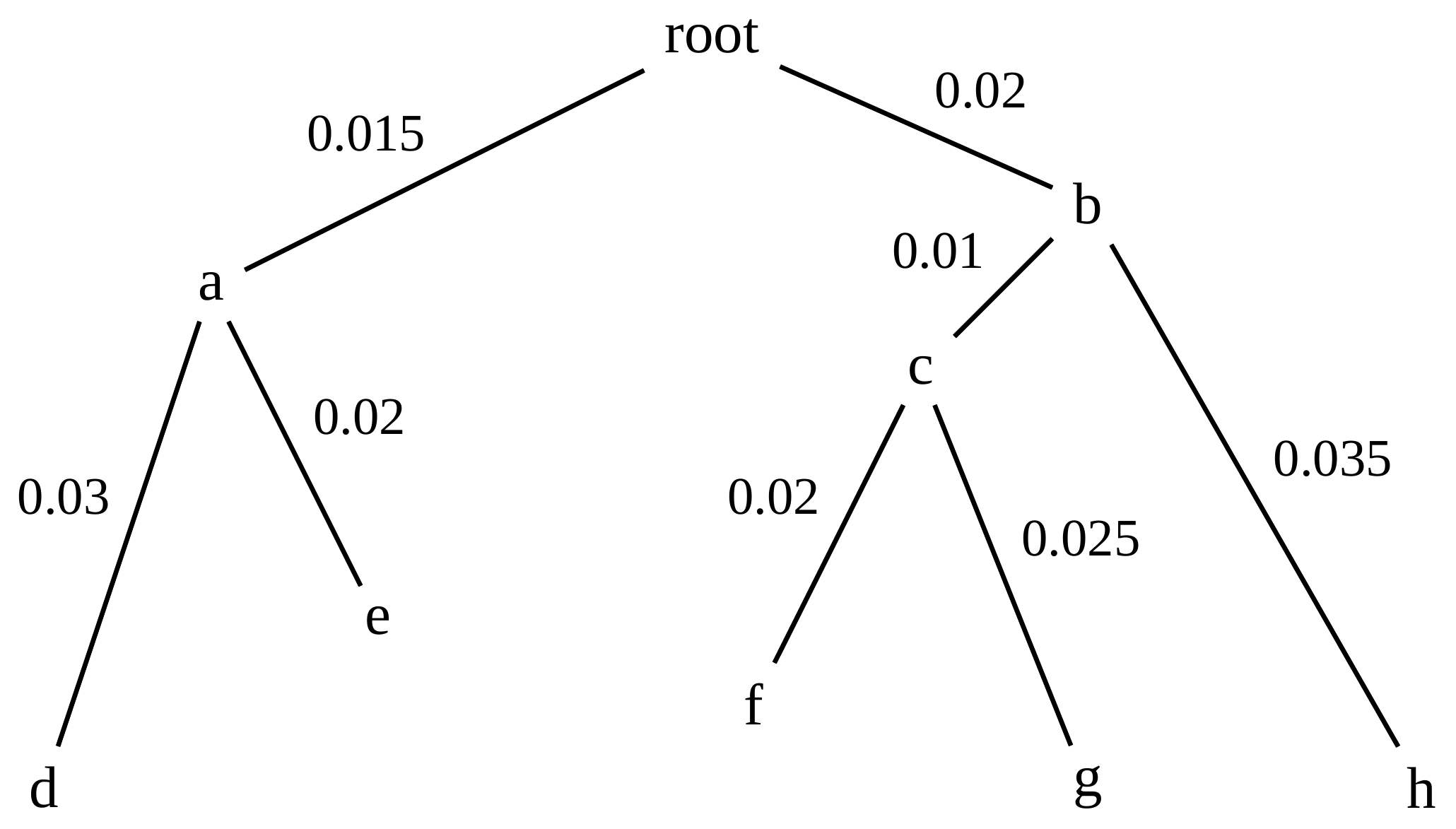
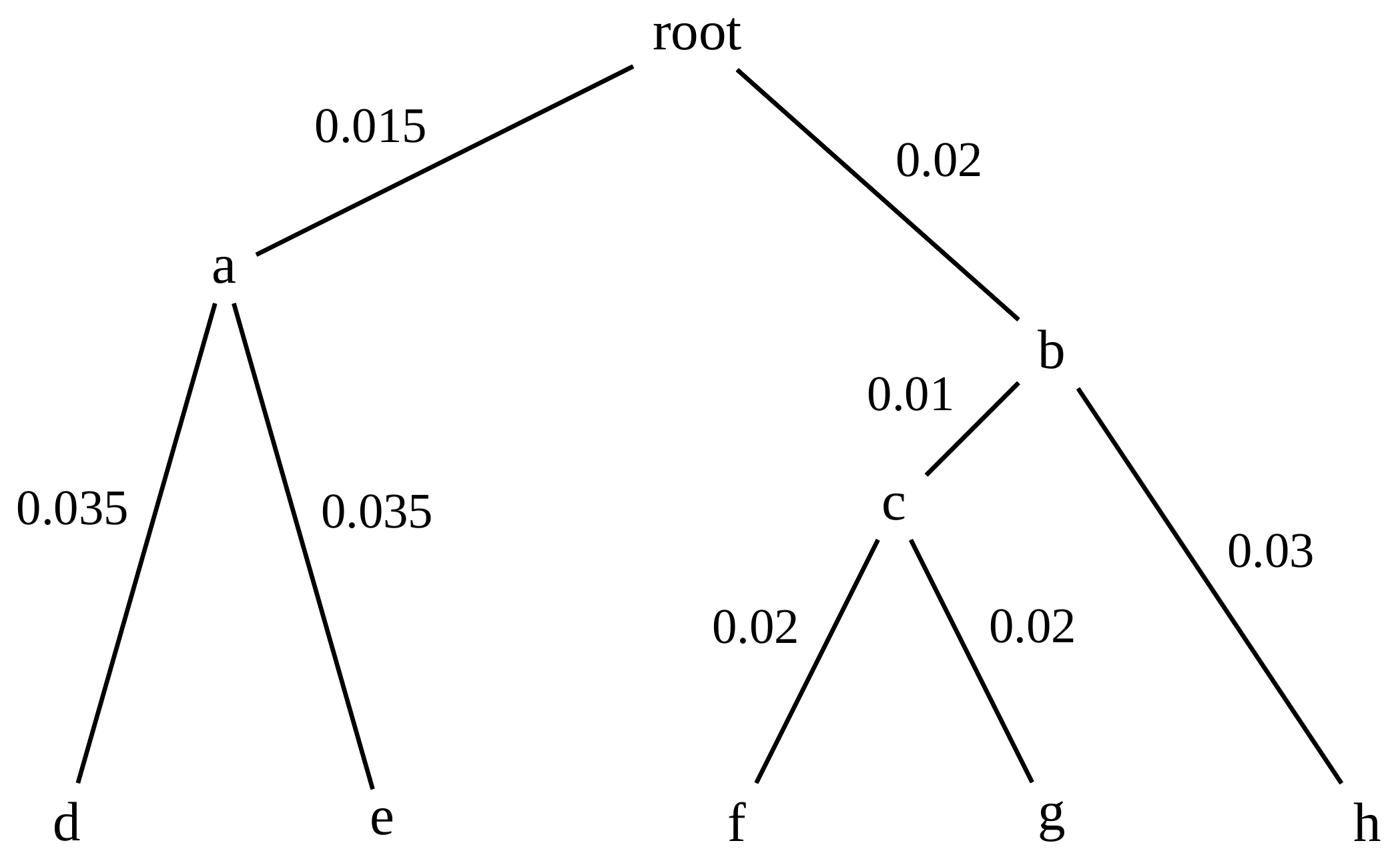
Rooted binary tree with branch lengths

Patristic Distances

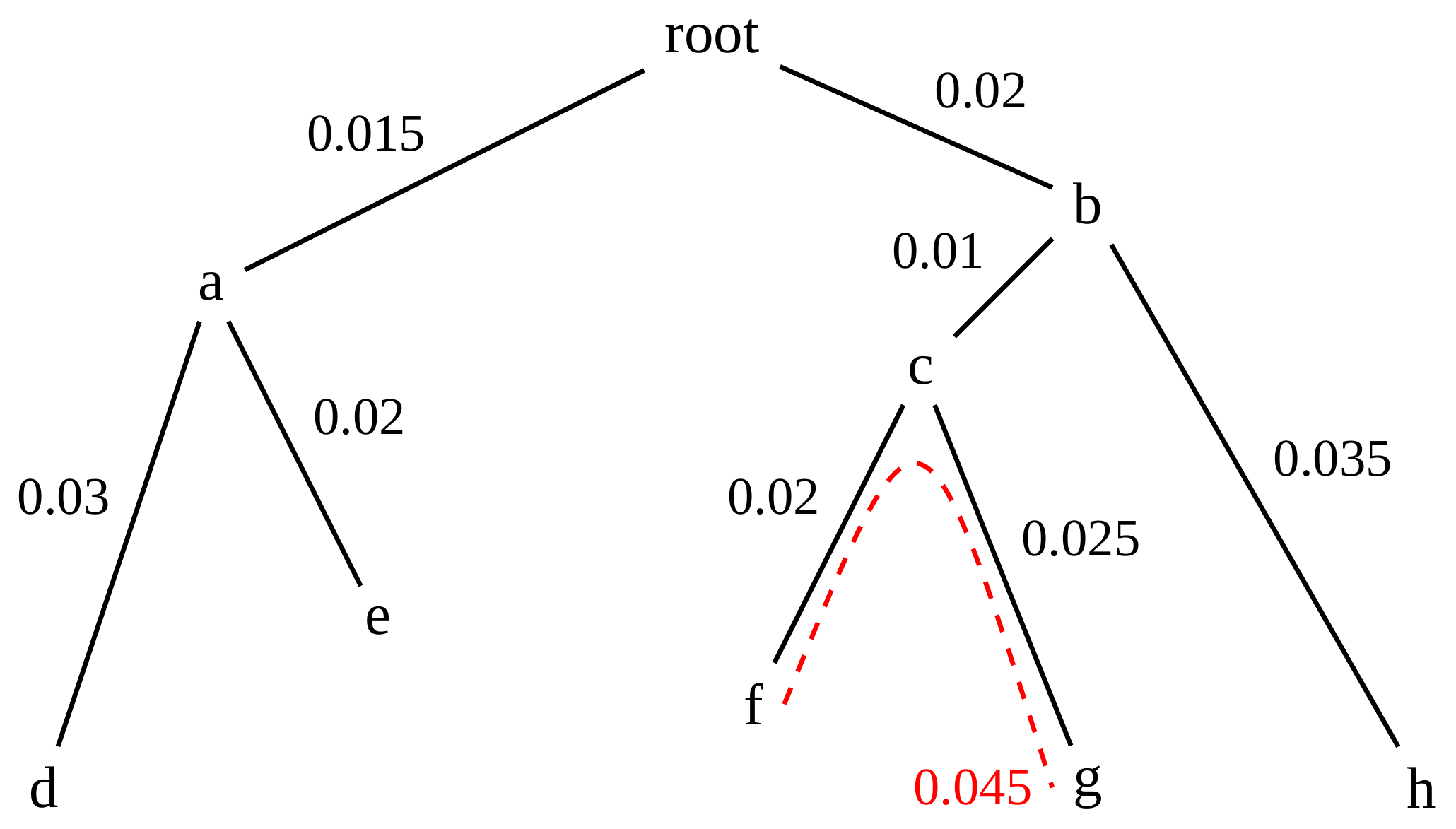
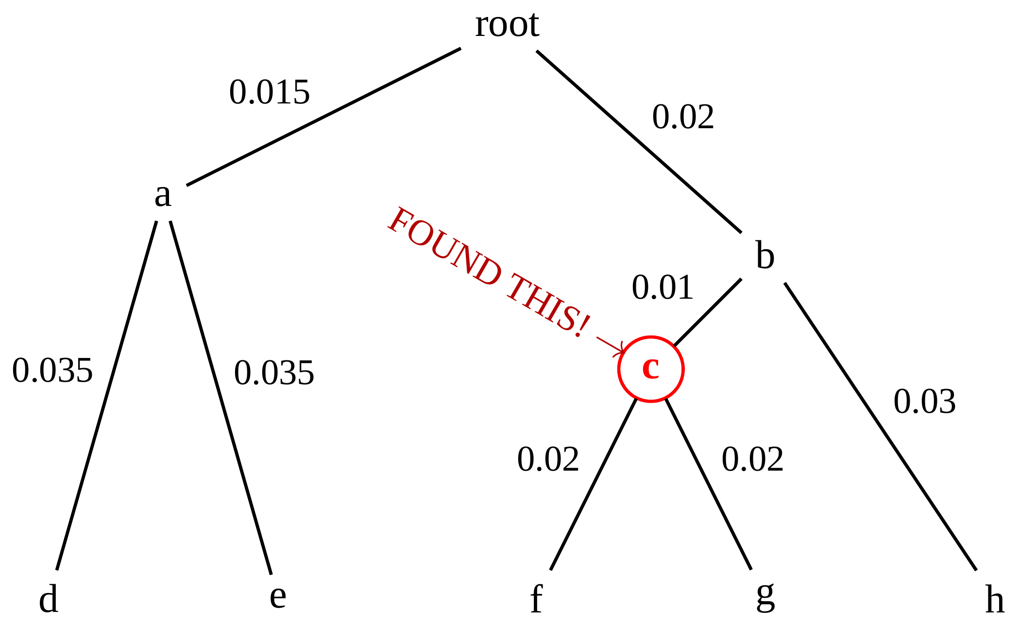
Patristic distance between tips f and g is 0.02 + 0.025 = 0.045 —

Patristic Distances

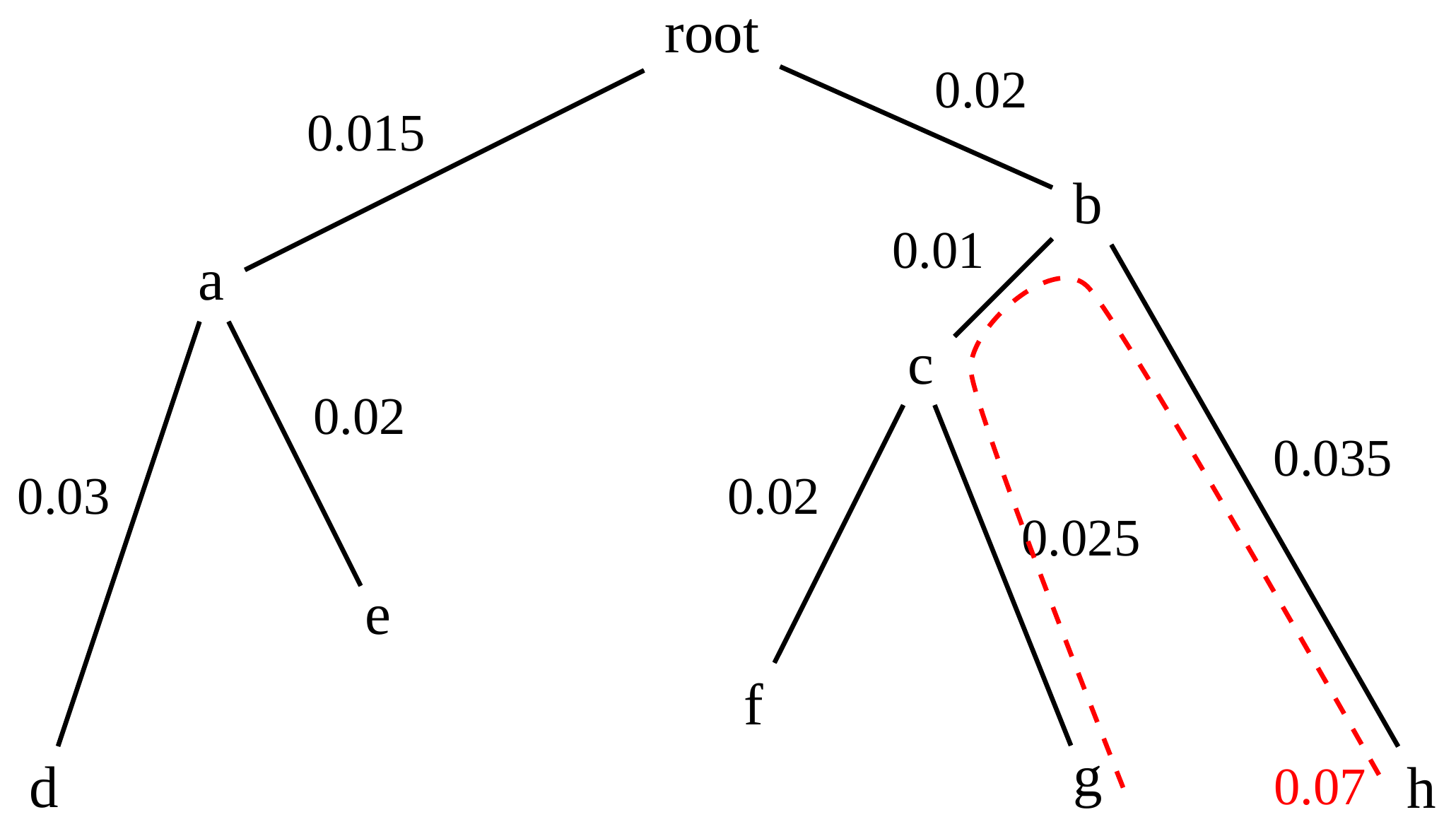
Patristic distance between tips g and h is 0.025 + 0.01 + 0.035 = 0.07 —

Patristic Distances

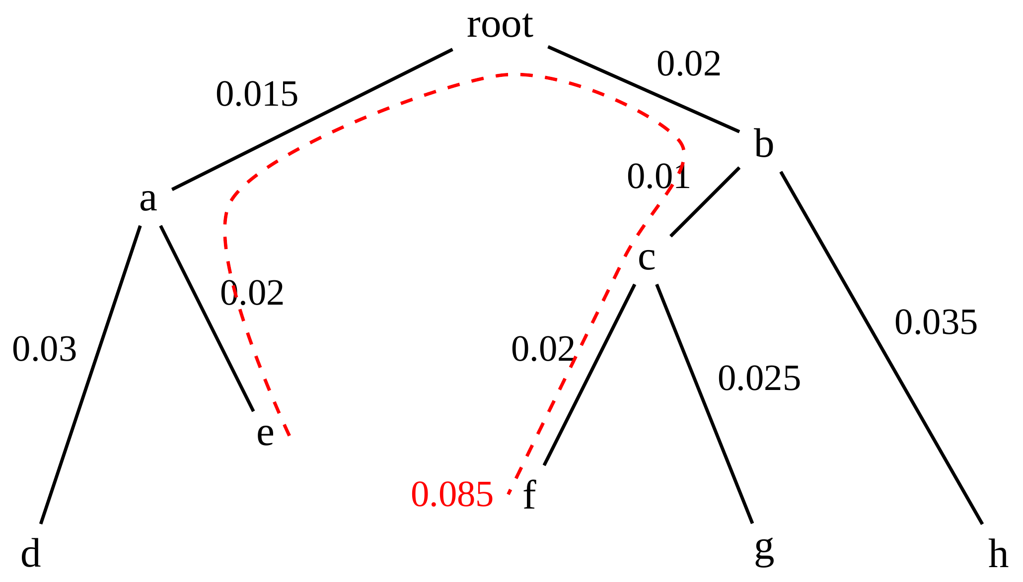
Patristic distance between tips e and f is 0.02 + 0.015 + 0.02 + 0.01 + 0.02 = 0.085

Tree-like distances are easy

A set of distances between the tips (taxa) that match the patristic distances of some tree is called tree-like.

Given tree-like distances, most tree construction methods will work.

Yes, most - not all!

Clock-like

The easiest possible distance data to work with are those where the distance from the root to every tip is the same.

Such trees (and the distances derived from them) are called ultrametric (that is, they have the same root-to-tip distance for every tip).

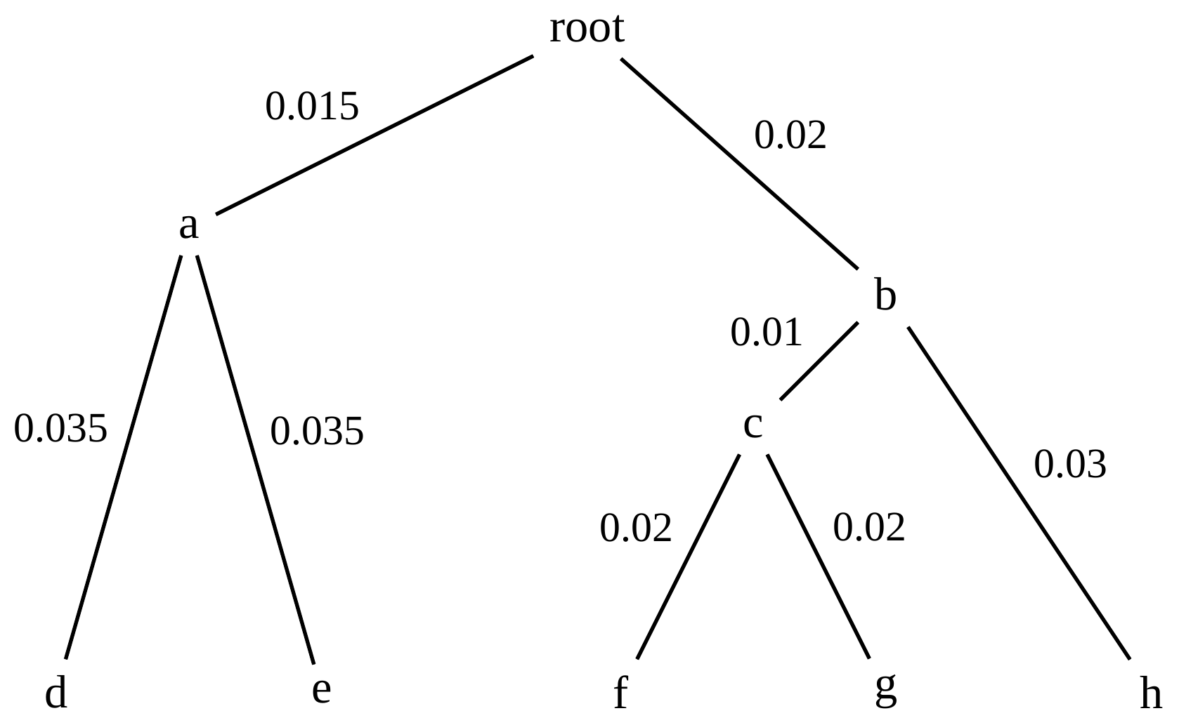
Clock-like

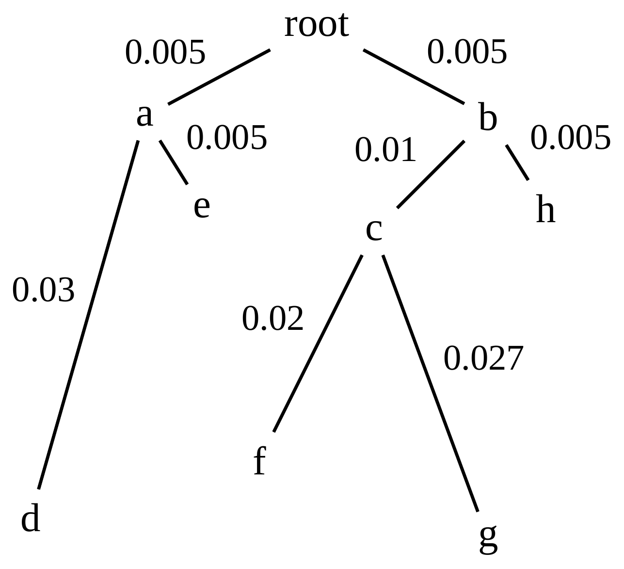
For example, suppose this is the true tree relating some species of interest, with actual branch lengths as labelled:

These distances are ultrametric

.pull-left[ .image-90[ ] ] .pull.right[

• The maximum root-to-tip distance is called the height of the tree.
• Here, the root-to-tip distances are all the same. A set of distances with this property is called ultrametric.
• If the distances represent evolutionary time accurately and all the tips are in the present, then we should expect this property.
• Reconstructing trees from ultrametric distances is super easy. ] —

These distances are ultrametric

.left-column40[ ] .right-column60[ Distance matrix: .center[ | | d | e | f | g | h | |:—:|:—:|:—:|:—:|:—:|:—:| |d | 0 | 0.07 | 0.1* | 0.1 | 0.1 | |e | 0.07 | 0 | 0.1 | 0.1 | 0.1 | |f | 0.1 | 0.1 | 0 | 0.04 | 0.06 | |g | 0.1 | 0.1 | 0.04 | 0 | 0.06 | |h | 0.1 | 0.1 | 0.06 | 0.06 | 0 | ] .reduce70[* Note; this is twice the root-to-tip distance.] ]

.pull-bottom[ Any ultrametric tree satisfies the three-point condition (for rooted trees): for any three tips x, y, z, the larger two pairwise distances of D(x, y), D(x,z), D(y,z) will be equal. ]

These distances are ultrametric

.left-column40[ ] .right-column60[ Distance matrix: .center[ | | d | e | f | g | h | |:—:|:—:|:—:|:—:|:—:|:—:| |d | 0 | 0.07 | 0.1 | 0.1 | 0.1 | |e | - | 0 | 0.1 | 0.1 | 0.1 | |f | - | - | 0 | 0.04 | 0.06 | |g | - | - | - | 0 | 0.06 | |h | - | - | - | - | 0 | ]
Since this is a symmetric matrix we usually just show half of it… ]

These distances are ultrametric

.left-column40[ ] .right-column60[ Distance matrix: .center[ | | e | f | g | h | |:—:|:—:|:—:|:—:|:—:|:—:| |d | 0.07 | 0.1 | 0.1 | 0.1 | |e | - | 0.1 | 0.1 | 0.1 | |f | - | - | 0.04 | 0.06 | |g | - | - | - | 0.06 | ]
… and only the non-zero entries. ]

The general approach

Our distances

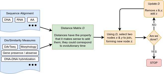
• We get distances from molecular sequences once they have been aligned.
• There are various ways to compare aligned sequences to obtain distances:
  • uncorrected “p-distance” – the proportion of sites that differ between the two sequences;
  • the Jukes-Cantor (JC69) correction, which takes into account of multiple character state changes through time;
  • The Hasegawa-Kishino-Yano (HKY85) model, which also allows for variation in nucleotide frequencies \(\pi_{A}, \pi_{C}, \pi_{G}, \pi_{T}\) as well as different transition/transversion rates;
  • and more.

Jukes-Cantor / JC69

This model has one single parameter, assuming that the base frequencies are each 25%: \(\pi_{A}=\pi_{G}=\pi_{C}=\pi_{T}=0.25\)

The rate matrix looks like this:
.image-40[ ]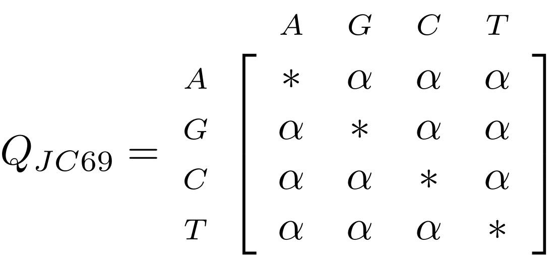
.reduce50[where the asterisk is a short-hand to make the row-sums equal 0.]

Under this model the expected number of substitutions between two sequences with a p-distance of \(p\) is \(\hat{d} = \frac{-3}{4}\ln\left(1-\frac{4}{3}p\right)\)

Hasegawa-Kishino-Yano / HKY85

This model allows for variation in nucleotide frequencies \(\pi_{A}, \pi_{G}, \pi_{C}, \pi_{T}\) as well as different transition/transversion rates using parameter \(\kappa\):

.image-40[ ]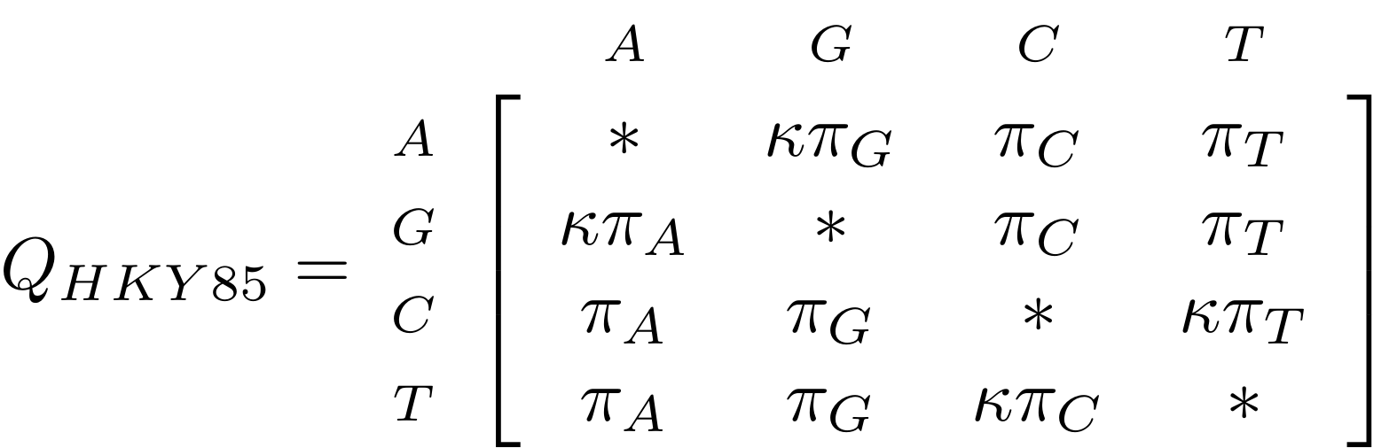

This model also allows for a correction to turn relative observed numbers of substitutions between the different bases into expected total number of substitutions between two sequences, but it is much more complex.

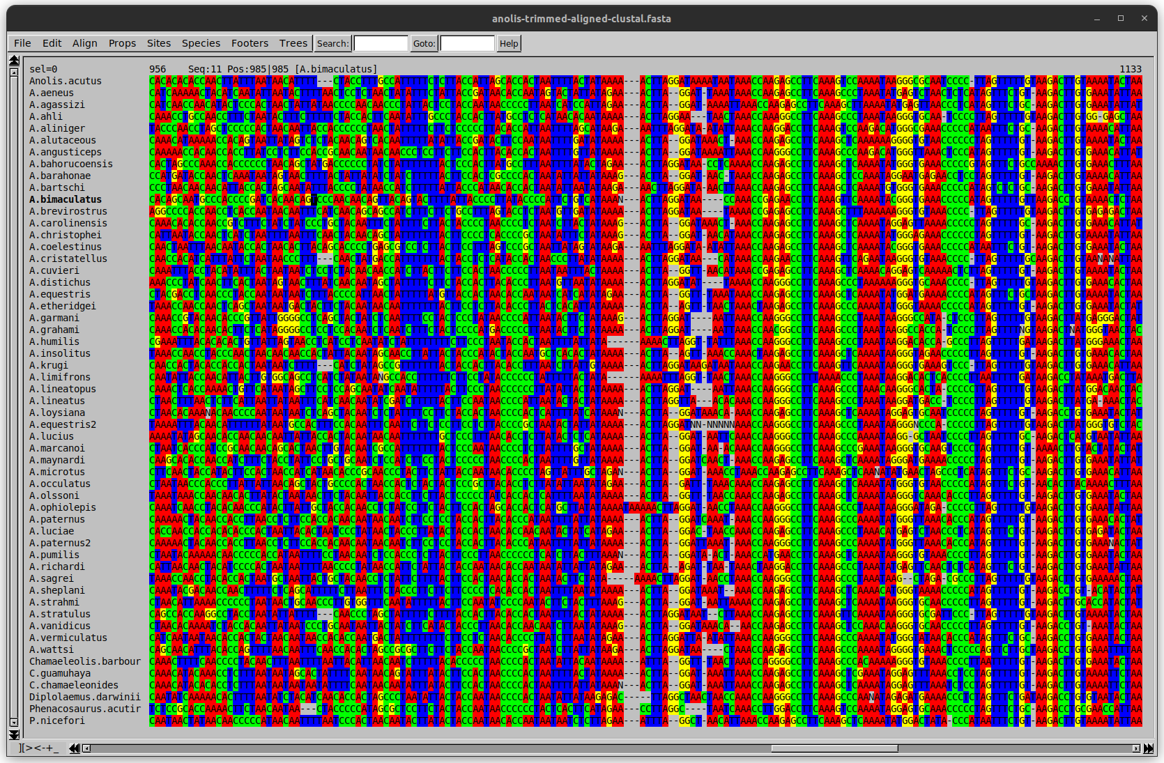
From alignment to distances

.left-column50[ ] .right-column50[

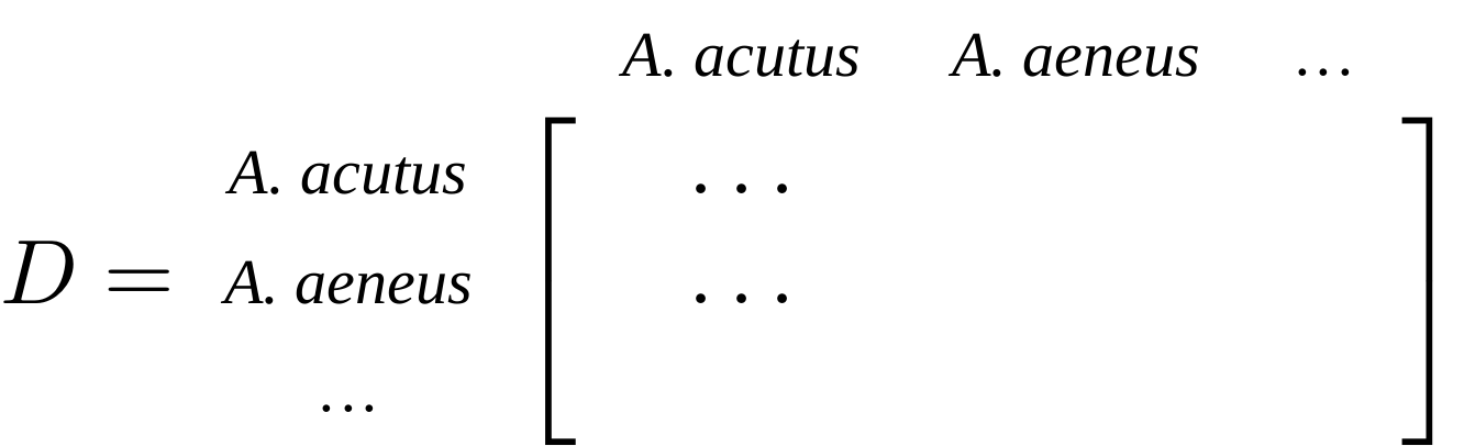
Once the alignment is complete, each pair of sequences is compared to give an estimated distance between them: this forms the distance matrix for tree building. ] —

Example

Ultrametric distances

The true tree

Original Distance Matrix

—

Original Distance Matrix

—




—

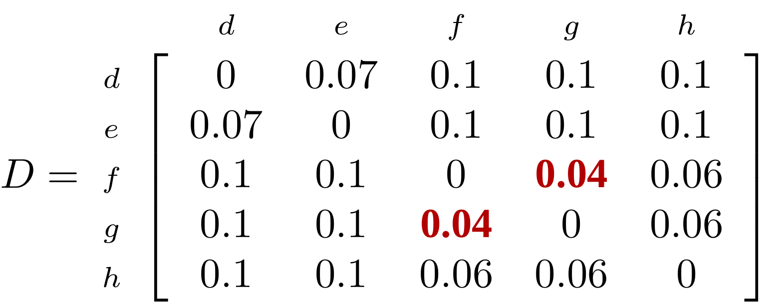
The distance between f and g D(f,g) is the sum of the branch lengths on the path between them. —

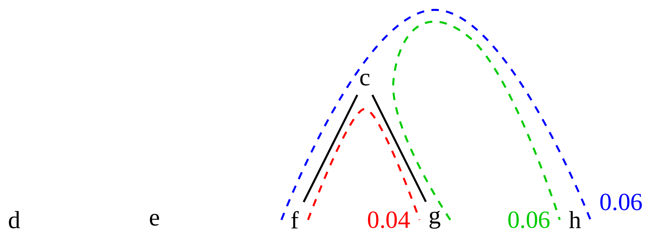
Similarly the distances D(f,h) and D(g,h) are the sum of branch lengths. —

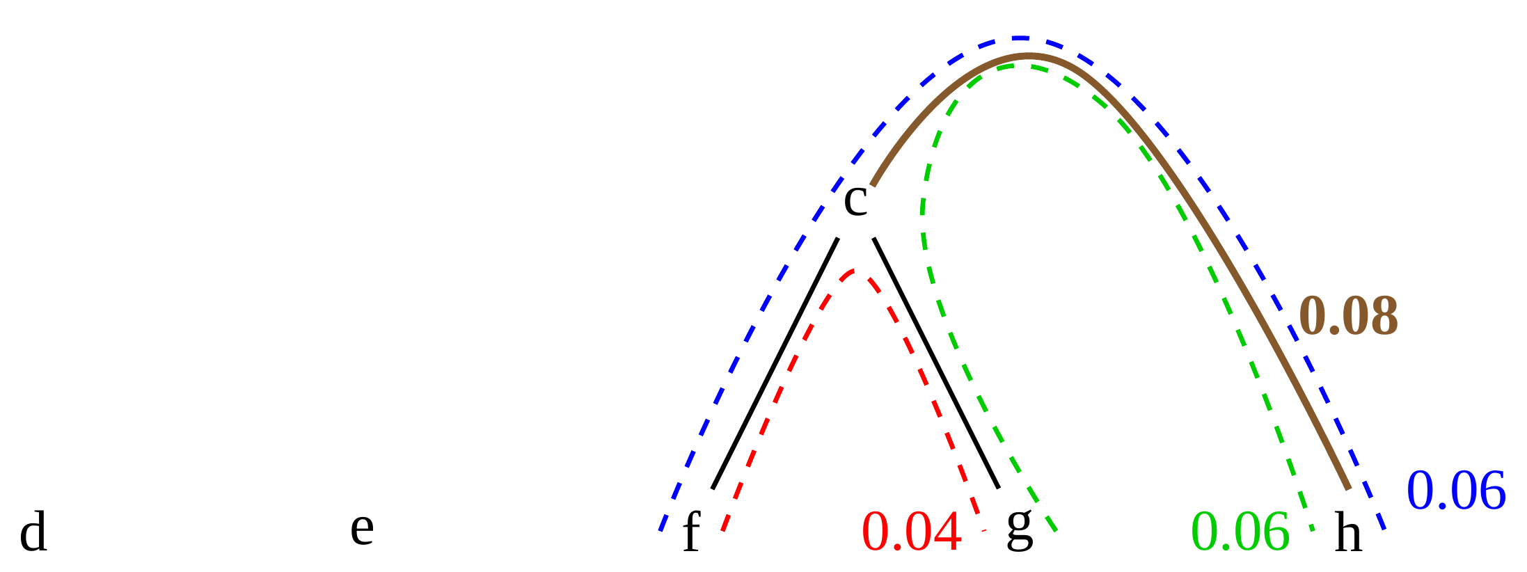
Therefore:
\(\mathbf{D(c,h)} = \frac{D(f,h)+D(g,h)-D(f,g)}{2}\)

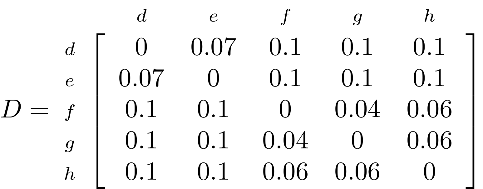
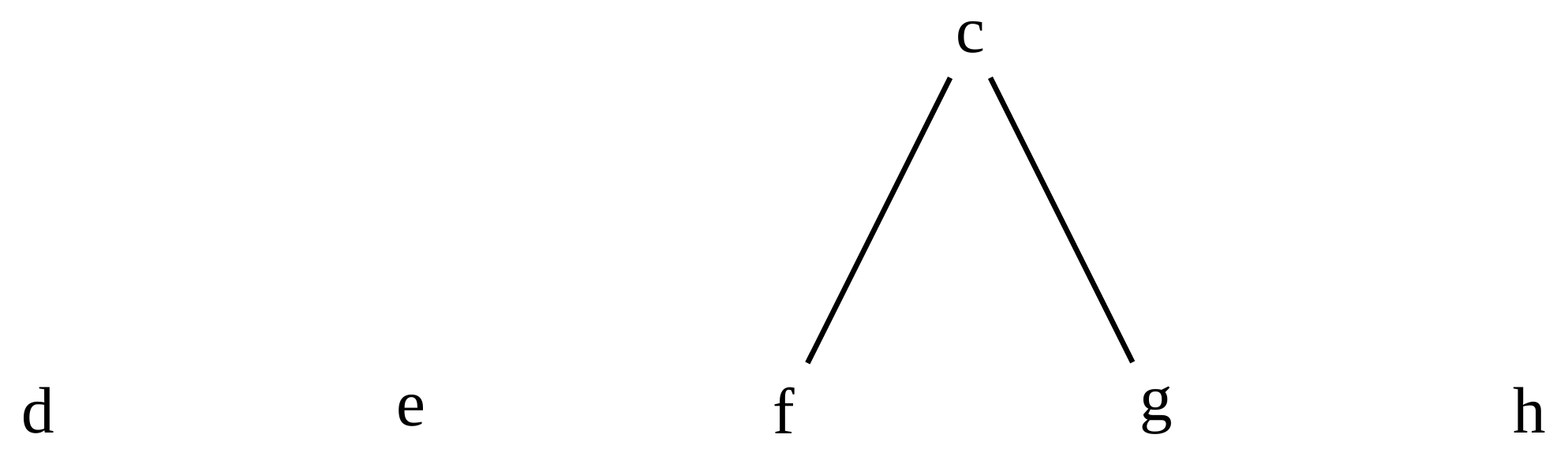
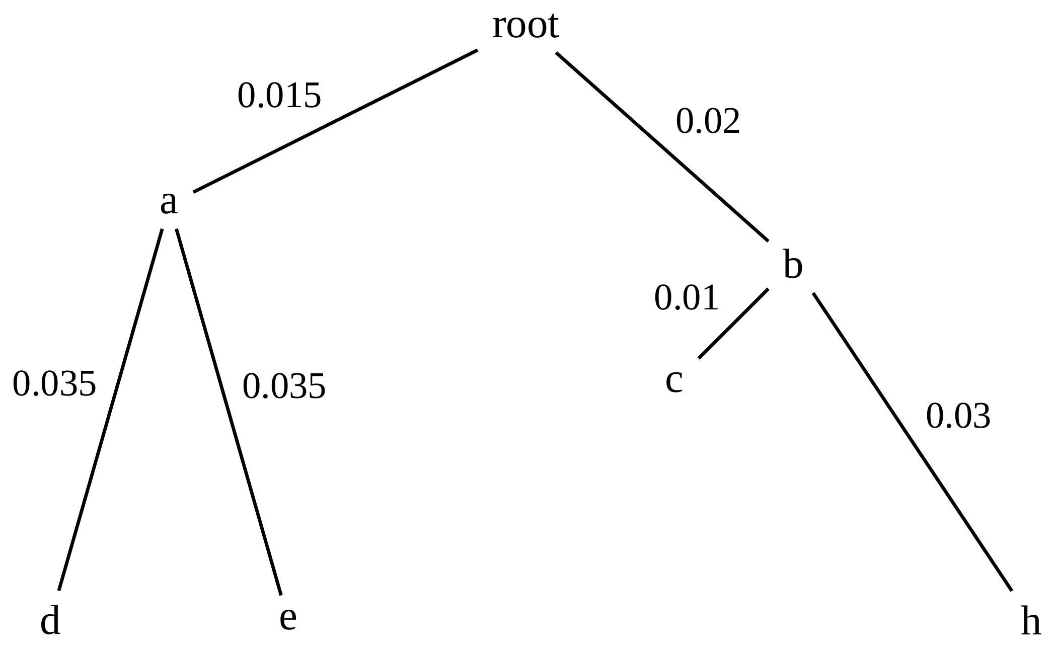
Forming the next Distance Matrix

We need to remove columns and rows f and g, and add new column and row c.

.image-75[ ]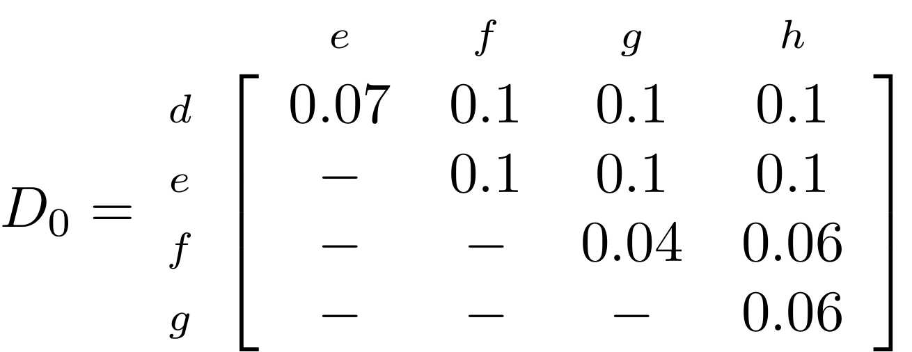

Forming the next Distance Matrix

The entries for D(f,d), D(g,d) etc get dropped.

.image-75[ ]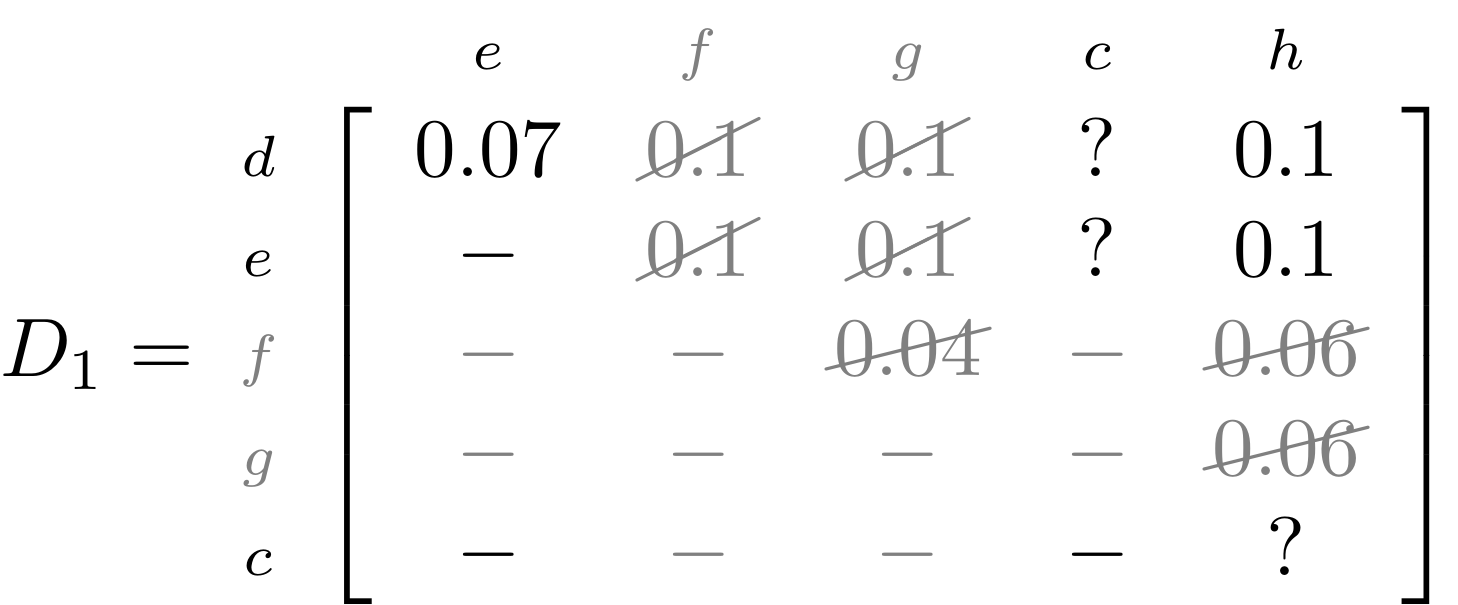

Forming the next Distance Matrix

We fill in the new entries using the formulae below:

.image-75[ ]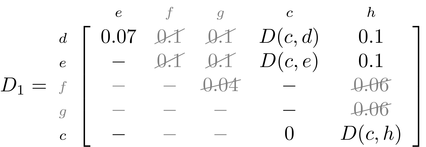

\(D(c,d) = \frac{1}{2}(D(f,d)+D(g,d)-D(f,g)) = \frac{1}{2}(0.1+0.1-0.04) = \mathbf{0.08}\) —

Forming the next Distance Matrix

We fill in the new entries using the formulae below:

.image-75[ ]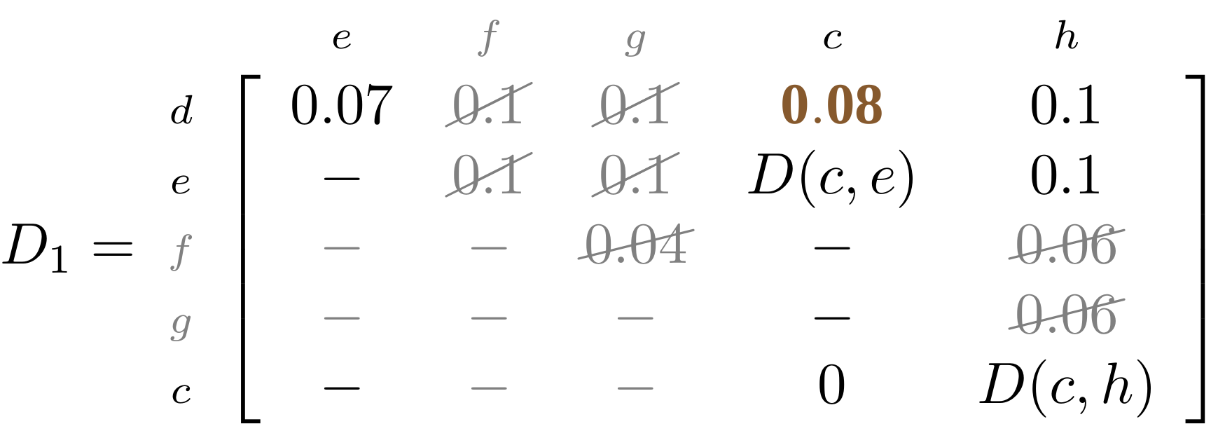

\(D(c,e) = \frac{1}{2}(D(f,e)+D(g,e)-D(f,g)) = \frac{1}{2}(0.1+0.1-0.04) = \mathbf{0.08}\) —

Forming the next Distance Matrix

We fill in the new entries using the formulae below:

.image-75[ ]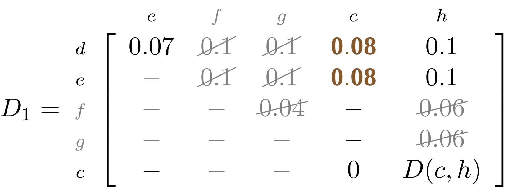

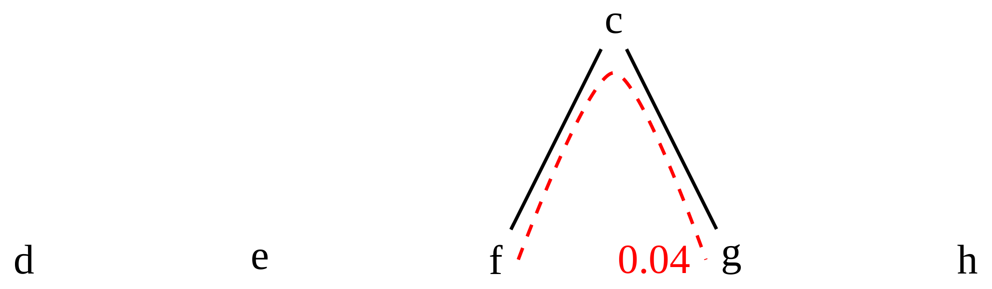
\(D(c,h) = \frac{1}{2}(D(f,h)+D(g,h)-D(f,g)) = \frac{1}{2}(0.06+0.06-0.04) = \mathbf{0.04}\) —

Forming the next Distance Matrix

.image-75[ ] —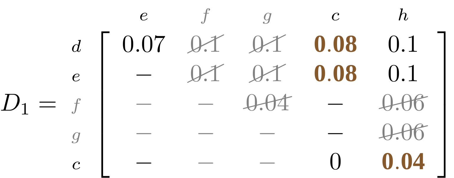

Forming the next Distance Matrix

Completed new distance matrix:

.image-50[ ]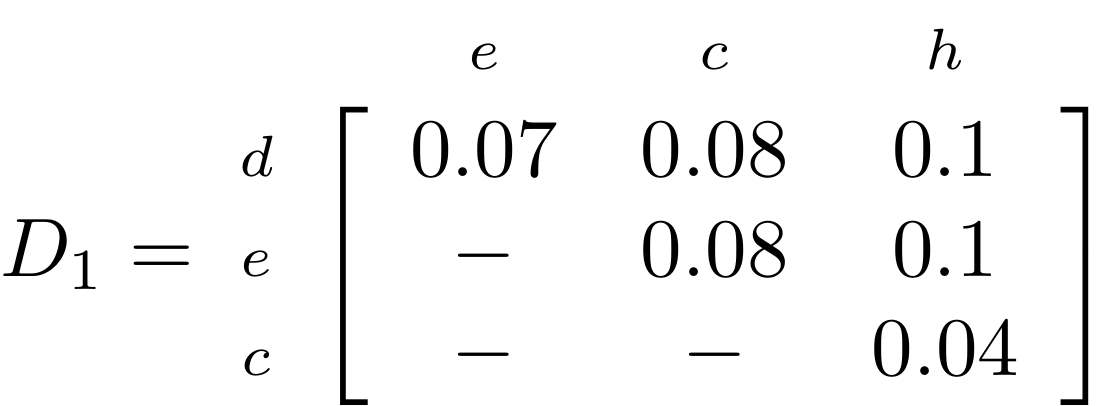

Now we have reduced the problem by one taxon / sequence: we repeat until we have just two more taxa to join and that will give us the root!

Non-clocklike trees

Losing the ultrametric property —

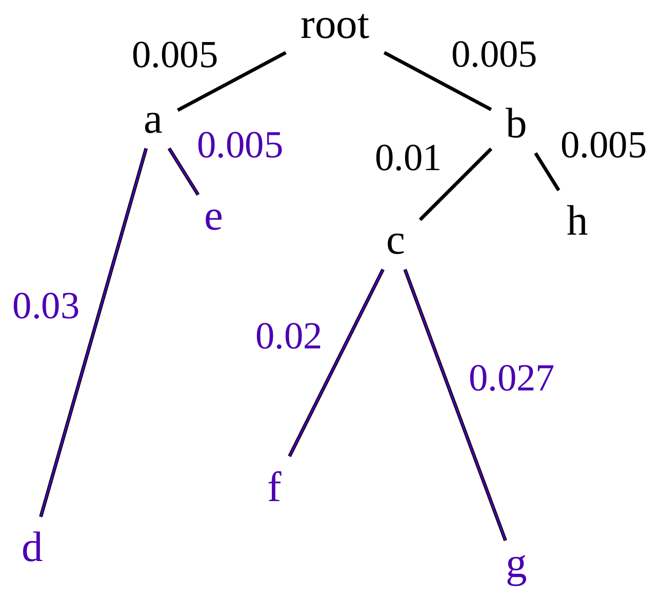
Not perfectly clock-like

Now suppose this is the true tree relating some species of interest, with actual branch lengths as labelled:

—

.left-column40[ ] .right-column60[ .image-75[ ]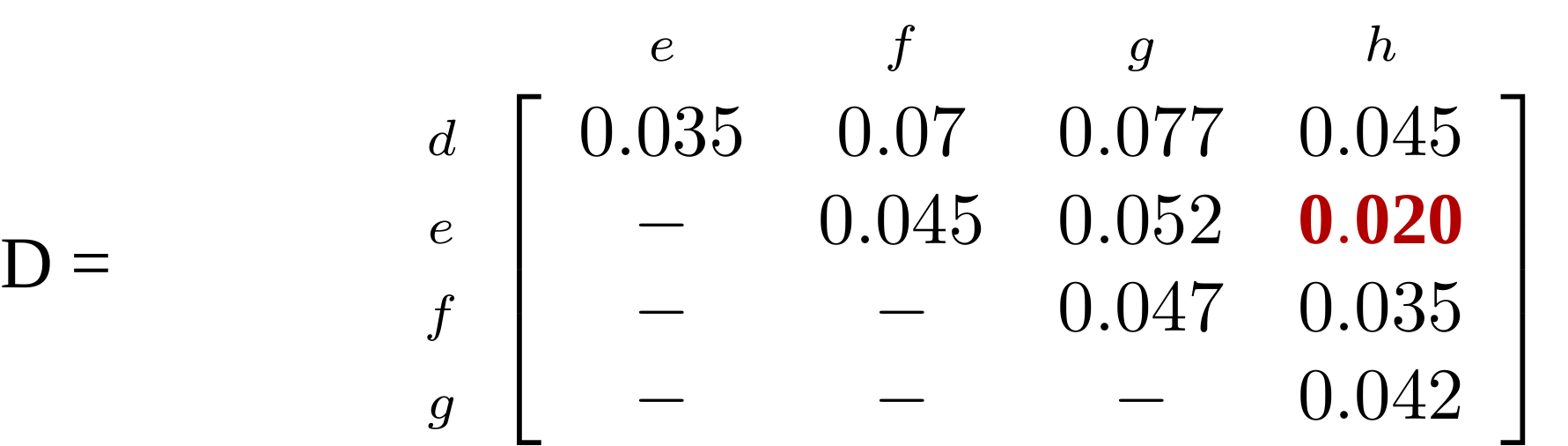
The smallest distance doesn’t match a true pair of siblings. ]

Neighbo[u]r-Joining

Neighbo[u]r-Joining solves this problem by accounting for the net divergence of node from the rest, so if distances are tree-like, even if they’re not ultrametric, it will get the tree right.

The formula for net divergence, with n taxa (i.e., an n x n distance matrix) is

\(r\_{i} = \frac{1}{n-2}\sum\_{j\neq i}D(i,j)\)

And the adjusted distance becomes

\(D^{\ast}(i,j) = D(i,j) - r(i) - r(j)\)

Adjusted distance matrix

Net divergences: .center[ | \(i\) | \(r(i)\) | |:—:|:——:| | d | 0.075666 | | e | 0.050666 | | f | 0.065666 | | g | 0.072666 | | h | 0.047333 | ]
Adjusted Distances:
.image-50[ ]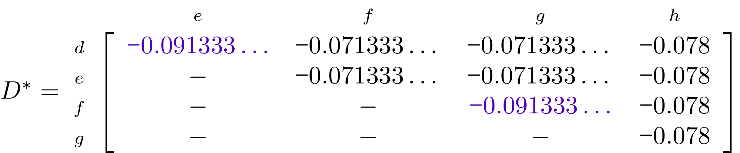

#Realistic data

Losing tree-like distances —

• Real data are not tree-like in general.
• We should adjust the final branch lengths that are found.
• One criterion is Minimum Evolution; this minimises the sum of squared differences (“ordinary least squares”; OLS) between the patristic distances, say G, from the tree and the original distances D:
  \(OLS = \sum\_{i,j}(D(i,j) - G(i,j))^{2}\)
  This assumes that the estimates are independent of each other, which clearly isn’t the case as the distances between tips in the tree often share parts of the paths between them.
  
  .reduce70[ Further reading: Denis and Gascuel: doi.org/10.1016/S0166-218X(02)00285-8. ]

Anolis tree with uncorrected p-distances

Anolis tree with JC69 distances

Anolis tree with HKY85 distances

Limitations

• A tree-building method will always give you a tree, even if the data didn’t come from one.
• There is no information on “next best” trees.
• There is no measure of “goodness” for the most part (though you could always quote the least squares error).
• Lastly, there is by default no going back on bad decisions: because NJ is a greedy heuristic, once the tree is finished, we stop. Luckily, we have programs like FastTree to do some adjustment!

#Thank you!

Next - estimating trees from alignments —

Thank you!